Note. The workflow described in this article applies to MotorXP-AFM 2.0 and later. In earlier versions the winding representation options and the analysis workflow differ.
Before you start. This article assumes you are familiar with the Lumped and Full winding models. If you are not, we recommend reading Part 1 — Winding Models: Lumped vs. Full first.
Introduction #
Dynamic Finite Element Analysis (Dynamic FEA) is the most powerful and accurate calculation method available. It accounts for rotor rotation, eddy currents, and higher harmonics, and relies on time-stepping transient FEA. In Dynamic FEA the current density has two components: one driven by the external voltage, and one induced by the changing magnetic field (eddy currents, skin effect, and proximity effect). As a result, when the Full winding model is used in Dynamic FEA, AC winding losses are included in the calculation.
Magnetostatic FEA uses prescribed stator winding currents with ideal sinusoidal or trapezoidal waveforms, via time-stepping magnetostatic FEA. The current density is imposed directly and only the static magnetic field is solved, so no eddy currents arise in the winding conductors. For this reason, in Magnetostatic FEA there is no significant difference between the Lumped and Full winding models — eddy currents, and therefore AC winding losses, are not captured. The Lumped model, however, significantly reduces simulation time.
AC losses can therefore be obtained as the difference between the stator winding loss computed with Dynamic FEA and the one computed with Magnetostatic FEA.
Table 2.1. Dynamic FEA vs. Magnetostatic FEA.
| Aspect | Magnetostatic FEA | Dynamic FEA |
| Current density | Imposed directly, uniform over the conductor | Voltage-driven + field-induced (non-uniform) |
| Eddy currents (skin / proximity) | Not captured | Captured |
| AC winding losses | Excluded | Included (with the Full model) |
| Winding model effect | Lumped ≈ Full (Lumped is faster) | Full required for AC losses |
| Simulation time | Short | Long |
Download the example projects #
The steps and results below are based on two ready-to-open MotorXP-AFM projects. Download them to reproduce the calculation:
Baseline losses in Magnetostatic FEA (without AC losses) #
In this mode you compute the copper losses caused only by the active (DC) resistance, with a uniform current-density distribution across each conductor.
Note. Magnetostatic FEA can be run in Design Studio or in the main MotorXP application.
Steps in Magnetostatic FEA (Design Studio Matlab/Standalone)
- Open the file lumpedWinding.mxa.
- Go to the Magnetostatic finite element analysis tab.
- In Current waveform, select Sinusoidal.
- In Current input method, select RMS supply current (or Peak supply current, or RMS current density) and enter the value.
- Set Advance angle and Mechanical speed.
- In Simulation setup, choose the required accuracy. This affects the Discretization error, which you can check in General Results after the run; it should not exceed a few percent.
click on image to enlarge
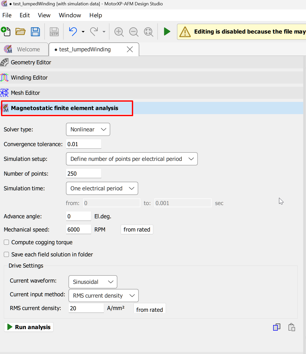
Figure 2.1. Magnetostatic FEA Tab (Design Studio).
- Click Run analysis.
click on image to enlarge
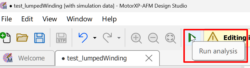
Figure 2.2. Magnetostatic FEA setup with a sinusoidal current source (Design Studio).
- When the run finishes, find Stator winding losses in Results.
click on image to enlarge
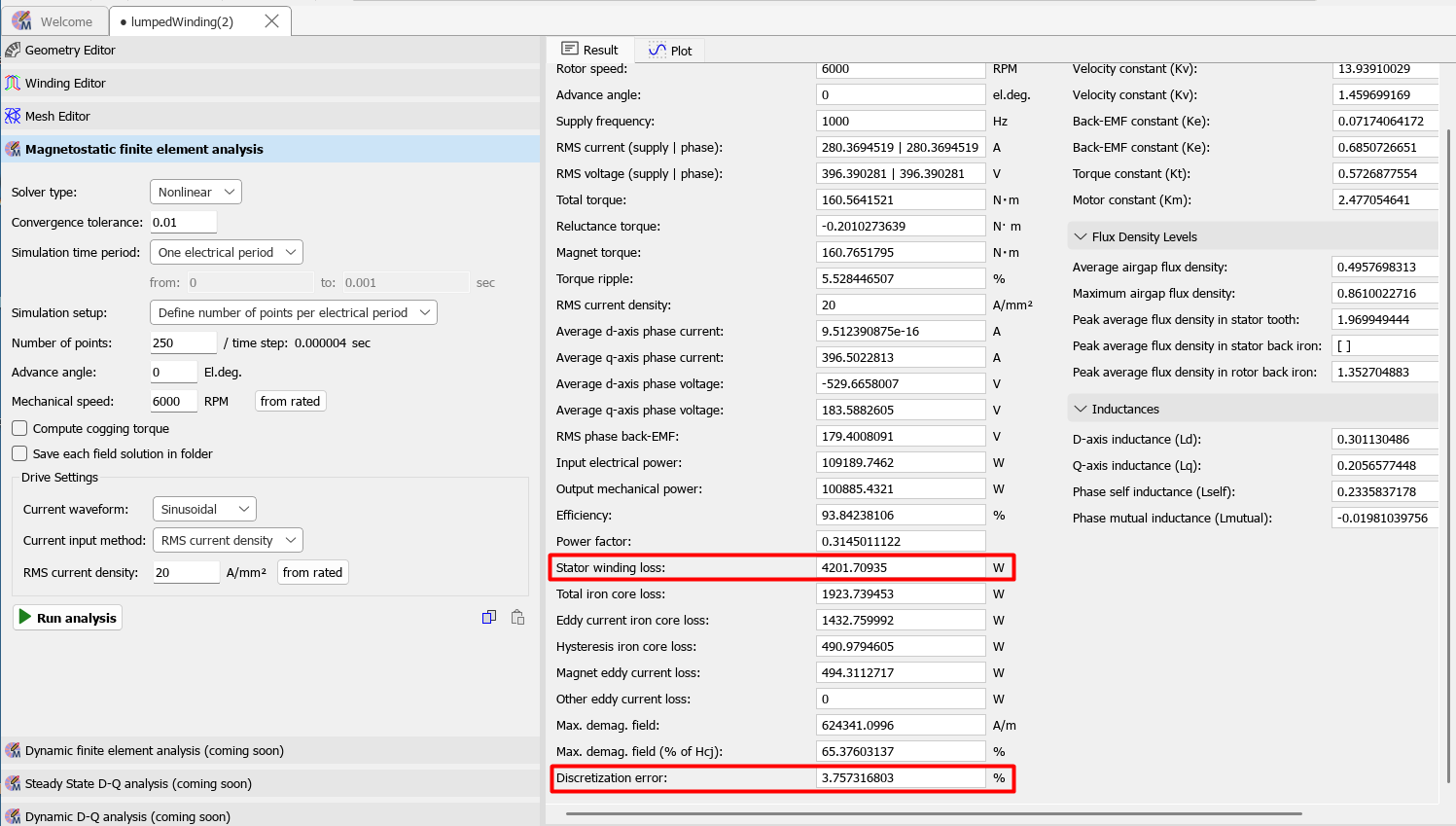
Figure 2.3. Stator winding losses reported in Results.
Steps in Magnetostatic FEA (MotorXP Matlab/Standalone)
You can find the sequence of steps at the following link:
Magnetostatic FEA in MotorXP-AFM: from the classic workflow to the new Design Studio.
Below, we present only the results. After the calculation is complete, find the Stator winding losses value in General Results.
click on image to enlarge
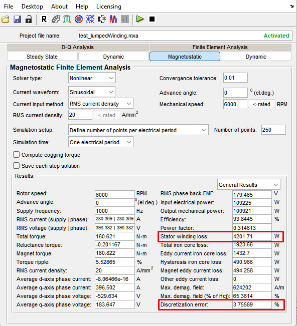
Figure 2.4. Stator winding losses in General Results.
Full losses in Dynamic FEA (with AC losses) #
In this mode you compute the copper losses caused both by the active resistance and by the changing magnetic field.
Model preparation
- Click Geometry Editor on the toolbar. The Design Studio window opens.
click on image to enlarge

Figure 2.5. Opening the Geometry Editor (Design Studio).
- Find the Coil geometry: line and select Full from the drop-down list.
- Set the following lines according to the winding data of the project.
click on image to enlarge
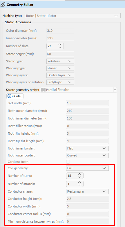
Figure 2.6. Switching the coil geometry to the Full winding model.
- Open the Mesh tab. To capture eddy currents (skin and proximity effects) correctly, the mesh in the conductor region must be sufficiently fine. Avoid over-refining the mesh, however — it substantially increases the computation time.
- Close the Design Studio window.
click on image to enlarge
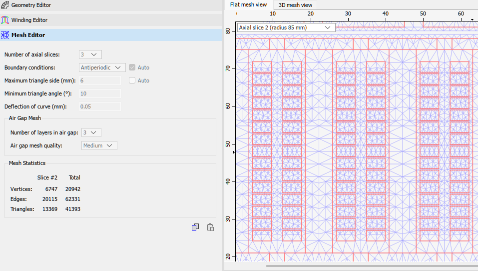
Figure 2.7. A sufficiently fine mesh in the conductor region for eddy-current capture.
Steps in Dynamic FEA
- Go to the Dynamic FEA tab.
- In Simulation settings, select Advanced. Apply an ideal sinusoidal current source — PWM substantially increases simulation time. Set Stator electrical circuit file to SinCurrentsSource (“3-phase current source”).
- Click Yes. The Simulation script file changes to simscript_sincurrentsource.m.
- Time step: use a sufficiently small step — at least 1/100 of one electrical period, where one electrical period equals 1 / (polePairs × rpm / 60). After the run, check the Discretization error in Time Average Quantities; it should not exceed a few percent.
- Simulation stop time: set it at least 20% longer than one electrical period of the supply frequency to exclude transient effects. Track the onset of steady state by the shape of the torque curve.
- Set Target RMS supply current, Target advance angle, and Speed — use exactly the same values as in Magnetostatic FEA. To track the eddy currents in the conductors over time, tick Save each field solution.
click on image to enlarge
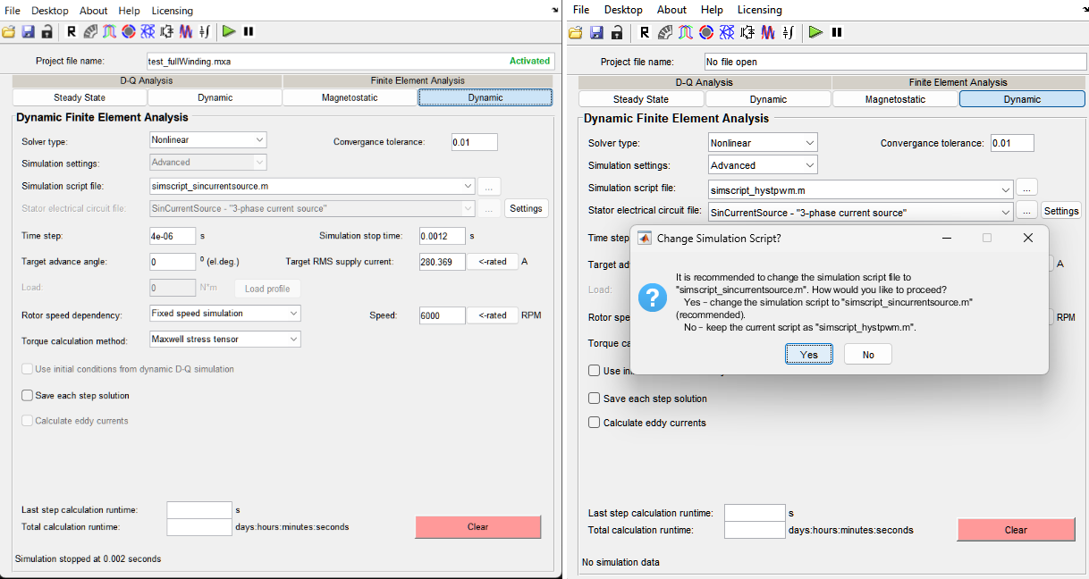
Figure 2.8. Source data (left) and selection of the 3-phase sinusoidal current source in Dynamic FEA (right).
- Click Start dynamic FE simulation and wait for the run to finish.
click on image to enlarge

Figure 2.10. Running the dynamic FE simulation.
- Plotting the graphs and setting their titles is done in the Plot Wizard (the button is located on the toolbar). In this example, two time plots are configured: the electromagnetic torque (in N·m) versus time, and the three phase currents Ia, Ib, Ic (in A) versus time.
click on image to enlarge
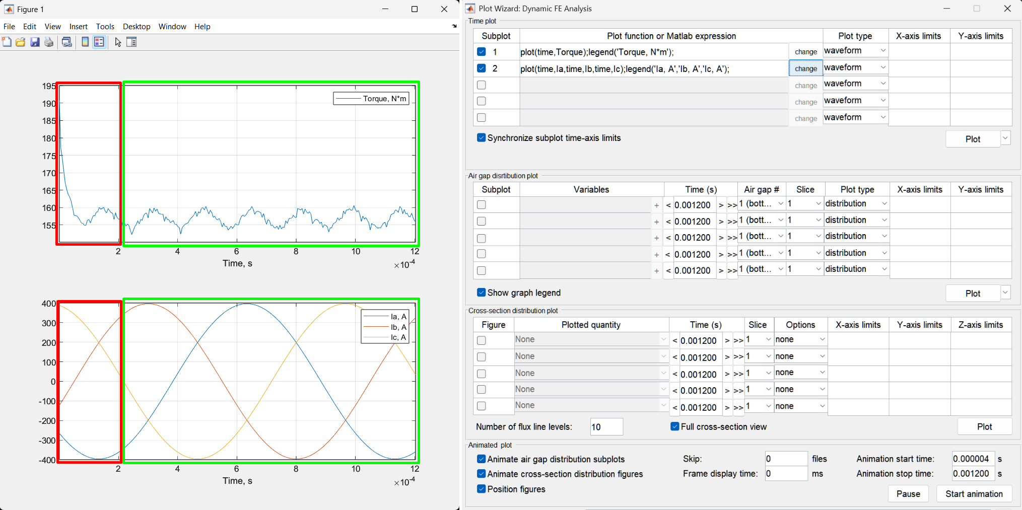
Figure 2.9. The torque curve settling into steady state.
In Figure 2.9, the red box on the torque curve highlights the transient process, which lasts approximately 0.0002 s, while one electrical period is 0.001 s and is highlighted by the green box.
- When the run finishes, click Time-averaged quantities in the main Dynamic FEA window.
click on image to enlarge

Figure 2.11. Opening the time-averaged quantities.
- Average the data over 1, 2, or 3 electrical periods (or set User choice).
- Find Stator winding losses in the list. These are the full winding losses, including the eddy-current losses.
click on image to enlarge
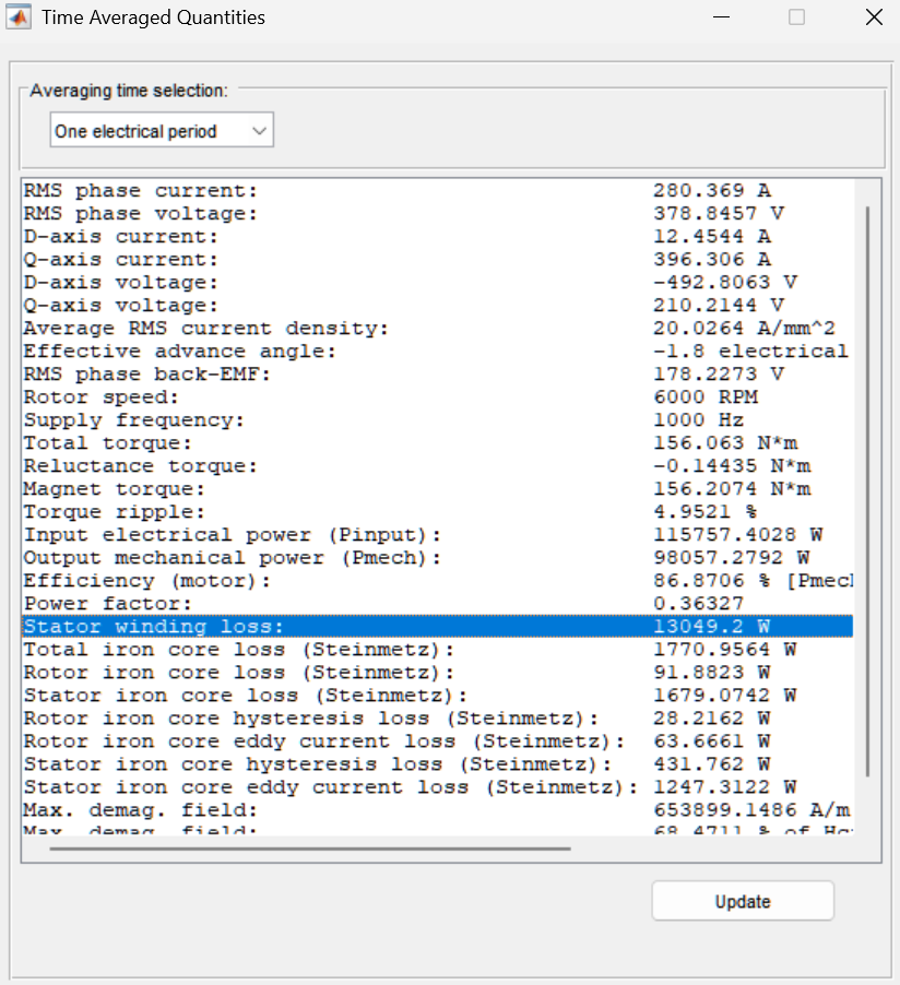
Figure 2.12. Full stator winding losses (including eddy-current losses) in Dynamic FEA.
Computing the AC losses #
AC losses are the difference between the stator winding loss from Dynamic FEA (Full winding model) and the stator winding loss from Magnetostatic FEA (Lumped or Full winding model):
AC losses = Pwinding (Dynamic FEA, Full) − Pwinding (Magnetostatic FEA)
Table 2.2. AC loss calculation for the example project.
| Quantity | Value |
| Stator winding loss — Dynamic FEA (Full model) | 13049.2 W |
| Stator winding loss — Magnetostatic FEA | 4201.71 W |
| AC losses (difference) | 8847.49 W |
| AC losses as a share of total winding loss | 67.8% |
In this example the AC losses reach 67.8% of the total stator winding loss, which shows how important it is to evaluate AC winding losses — especially at high speeds.
Visualizing the current-density distribution #
If you ticked Save each field solution, the magnetic field, loss, and current-density data are stored for every time step, so you can view animations and the distribution pattern at each computed time point. Without it you can still view these distributions, but only for the last computed time point.
Plotting the current density
- Click Plot Wizard on the toolbar.
click on image to enlarge

Figure 2.13. Button “Plot Wizard” on the toolbar.
- Select Cross-section distribution plots and plot Stator current density.
click on image to enlarge
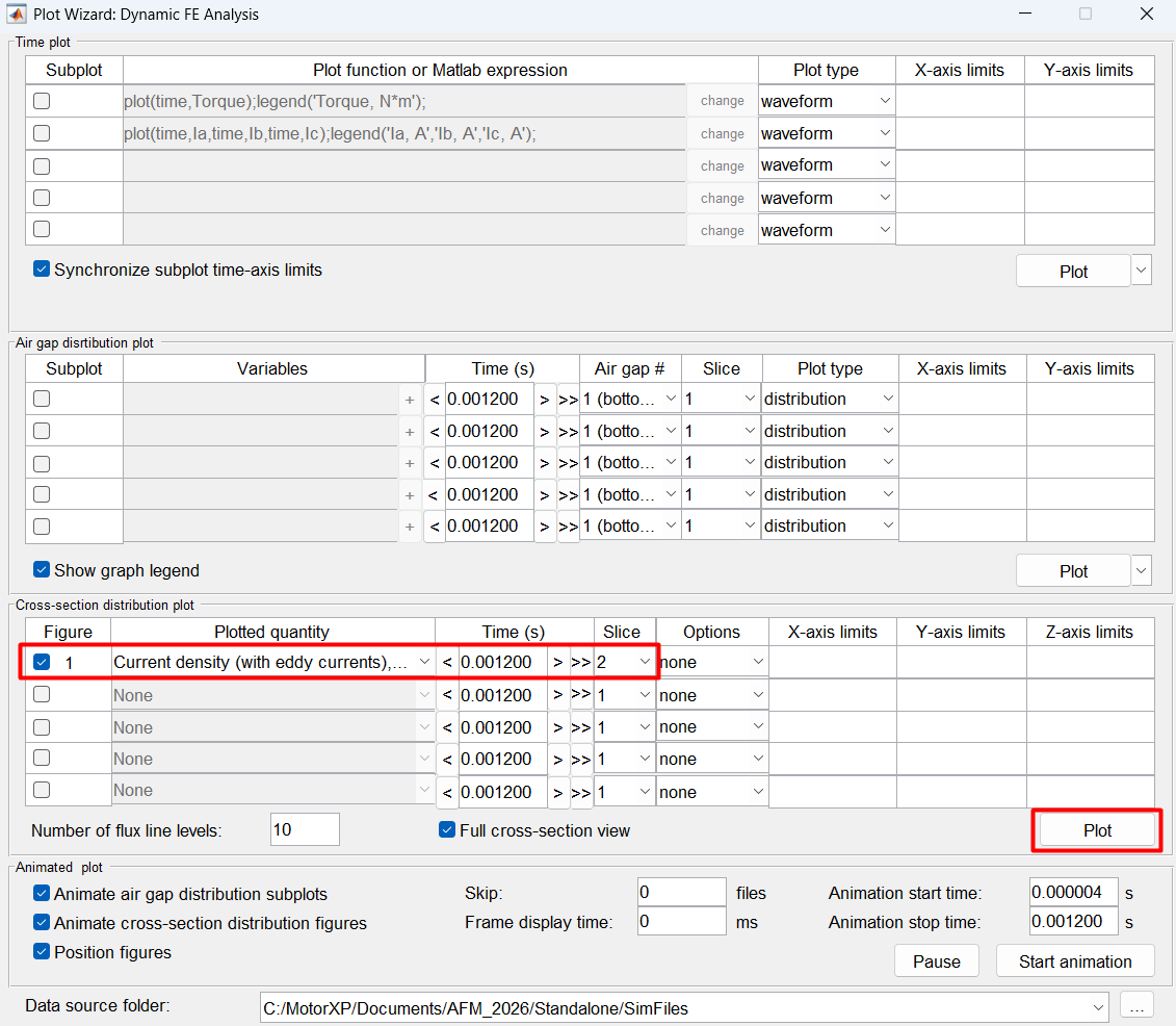
Figure 2.14. Plot Wizard: Dynamic FE Analysis.
In Dynamic FEA the current density is non-uniform across the conductor cross-section, whereas in Magnetostatic FEA it is uniform.
click on image to enlarge
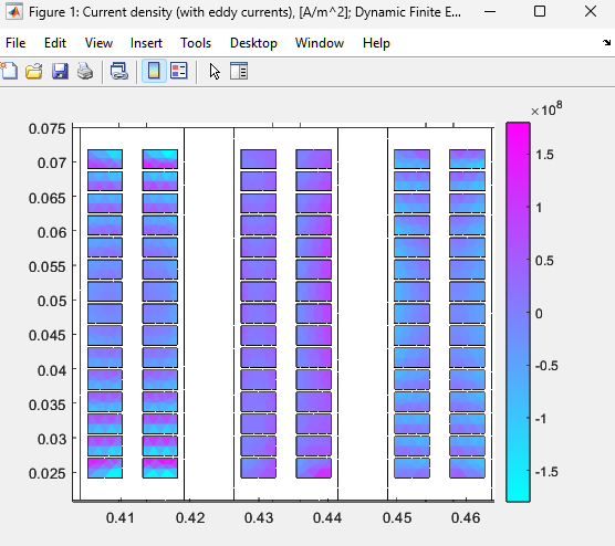
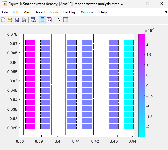
Figure 2.15. Stator current density with the Full winding model: Dynamic FEA (left) shows a non-uniform distribution across the conductor cross-section, while Magnetostatic FEA (right) shows a uniform distribution.


