Note. The workflow described in this article applies to MotorXP-AFM 2.0 and later. In earlier versions the winding representation options and the analysis workflow differ.
Before you start. This article continues Part 2 — Calculating AC Losses with Dynamic FEA. We recommend reading it first.
Introduction #
This section compares the results of four runs — Magnetostatic FEA and Dynamic FEA, each with the Lumped and the Full winding model — for the same operating point.
Magnetostatic FEA: Lumped vs. Full winding model #
Table 3.1. Magnetostatic FEA: Lumped vs. Full winding model.
| Parameter | Lumped | Full |
| Waveform | Sinusoidal | |
| Number of time steps per electrical period | 250 | 250 |
| Speed, rpm | 6000 | 6000 |
| Frequency, Hz | 1000 | 1000 |
| Current, Arms | 280.369 | 280.369 |
| Voltage, Vrms | 396.382 | 379.444 |
| Torque, Nm | 160.621 | 160.746 |
| Stator winding loss, W | 4201.71 | 4201.71 |
| Iron loss, W | 1923.66 | 1771.6 |
| Calculation time | 4 min 27 s | 10 min 9 s |
Dynamic FEA: Lumped vs. Full winding model #
Table 3.2. Dynamic FEA: Lumped vs. Full winding model.
| Parameter | Lumped | Full |
| Waveform | Sinusoidal current source | |
| Time step | 4e-06 s | 4e-06 s |
| Speed, rpm | 6000 | 6000 |
| Frequency, Hz | 1000 | 1000 |
| Current, Arms | 280.369 | 280.369 |
| Voltage, Vrms | 396.6121 | 378.8457 |
| Torque, Nm | 160.1608 | 156.063 |
| Stator winding loss, W | 4201.6958 | 13049.2 |
| Iron loss, W | 1942.9366 | 1770.9564 |
| Calculation time | 7 min 15 s | 34 min 55 s |
Comparison of results #
For Magnetostatic FEA with the Lumped model (Table 3.1) and Dynamic FEA with the Lumped model (Table 3.2), the results are practically identical; the only difference is the calculation time, which for Dynamic FEA is almost twice that of Magnetostatic FEA.
The Dynamic FEA run used a sinusoidal current source, which feeds an ideal sinusoidal current directly into the stator phase windings. This lets the simulation start straight in the steady state, substantially shortening the Dynamic FEA runtime.
As Table 3.2 shows, the Dynamic FEA runtime with the Full model is almost 5× that with the Lumped model. At the same time, the stator winding loss with the Full model is 3.1× higher than with the Lumped model. This is because Dynamic FEA with the Full model computes the full copper loss — the loss on the active resistance (DC losses) plus the loss from eddy currents (AC losses). The same effect explains the roughly 3% difference in torque.
Because the Full model places each conductor individually, the Dynamic FEA simulation also captures the skin effect and the proximity effect in the conductors, which affects the copper loss.
The current-density distribution over the winding cross-section is compared below for Magnetostatic FEA (Lumped and Full) and Dynamic FEA (Lumped and Full).
click on image to enlarge
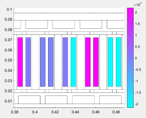
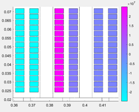
Magnetostatic FEA — Lumped (left) and Full (right)
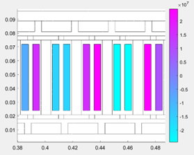
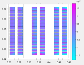
Dynamic FEA — Lumped (left) and Full (right)
Figure 3.1. Comparison of the current-density distribution over the winding cross-section.
The figures show that Dynamic FEA with the Full model produces a non-uniform current-density distribution in the slot and across the conductor cross-sections — precisely the result of the skin and proximity effects. The distribution also has an angular, faceted look that follows the finite-element mesh; refining the mesh would make it smoother.
In Dynamic FEA with the Lumped model there are no skin or proximity effects, because the conductor is represented as a single equivalent object. In Magnetostatic FEA the stator winding currents are prescribed directly, so no eddy currents arise in the winding conductors.


