Note. The workflow described in this article applies to MotorXP-AFM 2.0 and later. In earlier versions the winding representation options and the analysis workflow differ.
Before you start. This article continues Part 3 — Comparing the four cases: Magnetostatic and Dynamic FEA with the Lumped and Full winding models. We recommend reading it first.
Introduction #
MotorXP-AFM offers two ways to realize a sinusoidal current in Dynamic FEA. If you need a clean sinusoidal current without PWM ripple, use the advanced simulation script file with the Sinusoidal current source. If you want to study the influence of the control system and the higher harmonics, use the standard option with space-vector PWM and an inverter.
By default, Dynamic FEA models an electric machine connected to an inverter. The current is not imposed directly as an ideal source — it is formed by the control system.
Before running Dynamic FEA with space-vector PWM, we recommend running a Dynamic D-Q Analysis first. It serves as a preparatory step for the Dynamic FEA: it computes the initial conditions and speeds up the simulation.
click on image to enlarge
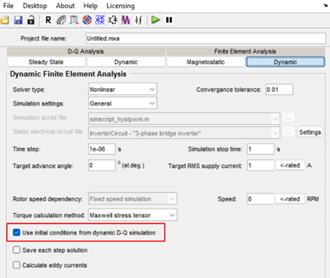
Figure 4.1. The “Use initial conditions from dynamic D-Q simulation” option in Dynamic FEA.
Download the example project #
The steps and results below are based on a ready-to-open MotorXP-AFM project. Download it to reproduce the calculation:
Configuring the inverter and PWM (Drive Settings) #
Before running the Dynamic DQ analysis, configure the inverter and the PWM type in the Drive Settings window. Click Drive Settings on the toolbar.
click on image to enlarge

Figure 4.2. The Drive Settings button on the toolbar.
The Drive Settings window opens.
click on image to enlarge
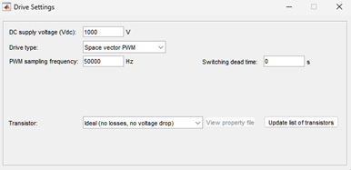
Figure 4.3. The Drive Settings window.
Configure the parameters in the Drive Settings window
- DC supply voltage (Vdc): set the source voltage. For an initial calculation with star-connected phases, you can take
\[ V_{dc} = \sqrt{6}\;V_{ph,\,rms}, \]
where the RMS phase voltage \( V_{ph,\,rms} \) can be read from Time Averaged Quantities in the Dynamic DQ Analysis.
click on image to enlarge
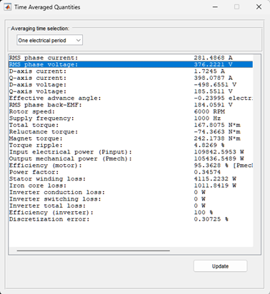
Figure 4.4. Reading the RMS phase voltage from Time Averaged Quantities to set Vdc.
- Drive type: select the PWM type. This example uses Space vector PWM.
- Transistor: to account for inverter losses and the transistor voltage drop, select a specific type (MOSFET or IGBT) and set its parameters. If you select ideal (no losses, no voltage drop), losses and voltage drop are ignored.
- Switching dead time: typically 0 to 5 µs.
- PWM sampling frequency: you can take it as 50× the fundamental frequency, 50·f (Hz) (if the PWM frequency is known, use it).
- Close the Drive Settings window.
Building the Dynamic DQ model #
- Go to Dynamic DQ Analysis.
- Current and angle ranges: set Maximum RMS current, Current step, and Advance angle step to cover all the operating points.
- Number of rotor positions: use at least 2 rotor positions. This averages the DQ-model parameters and compensates their variation due to the cogging torque during rotation.
- Include iron losses: tick this to account for iron losses. Note that it significantly increases the model parametrization time.
- Click Build DQ model.
click on image to enlarge
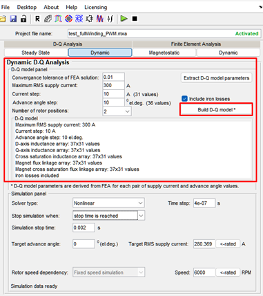
Figure 4.5. Building the D-Q model.
- Wait for the run to finish. The DQ-model build time depends on the number of parametrization points.
Configuring and running the Dynamic D-Q Analysis #
- Go to Dynamic DQ Analysis.
- Solver type determines how the D-Q model parameters are interpolated. Nonlinear is the recommended solver for reliable results, but
Linearized is usually sufficient (provided enough current/angle pairs were used when building the D-Q model). Linear is suitable only for a coreless (ironless) motor or when saturation is negligible. - Time step must be small compared with the PWM sampling period. Recommended procedure:
- compute the fundamental frequency f (Hz) = polePairs·rpm/60;
- take the PWM frequency fpwm = 50·f (Hz) (use the known value if available);
- compute the PWM period PeriodPWM = 1/fpwm;
- take the time step at least 50× smaller than the PWM period: PeriodPWM/50;
- the Discretization error indicates the accuracy — monitor it in Time Average Quantities after the run; it should not exceed a few percent. Adjust the time step if needed.
- Stop simulation when: stop by time (Simulation stop time) or automatically at steady state. If you use Simulation stop time, set it to at least two electrical periods of the fundamental, 2·(1/f), to exclude transient effects.
- Set Target RMS supply current and Target advance angle. For the Current hysteresis PWM and Space vector PWM drives, the control algorithm automatically adjusts the inverter voltage to hold the specified current and advance angle.
- Rotor speed dependency. Fixed speed simulation: the speed is fixed — specify only its value. Variable speed simulation: the speed varies with the electromagnetic torque and the load.
- Click Start Dynamic DQ simulation on the toolbar.
click on image to enlarge
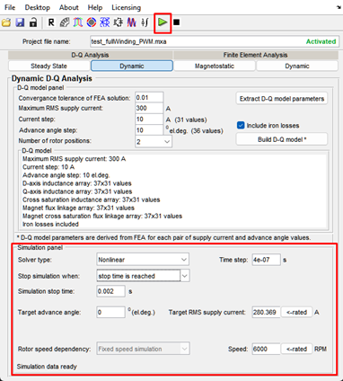
Figure 4.6. Starting the Dynamic DQ simulation.
After the run, analyze the results in Time-averaged quantities and Plot Wizard.
click on image to enlarge

Figure 4.7. Opening Time-averaged quantities and Plot Wizard after the DQ run.
In Time-averaged quantities you can view the parameters averaged over 1, 2, or 3 electrical periods, or over a user-defined time. Here you can check whether the Target RMS supply current and Target advance angle are reached, along with the discretization error. If these are within range, you can move on to the Dynamic FEA simulation.
click on image to enlarge
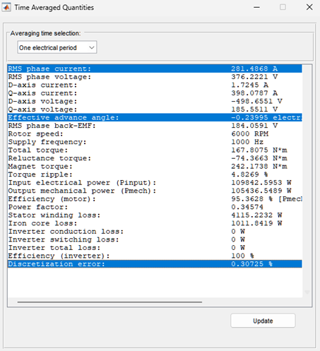
Figure 4.8. Time-averaged quantities in the Dynamic DQ Analysis.
In Plot Wizard you have access to currents, voltages, torque, speed, powers, losses, and DQ-model parameters (inductances, flux linkages). Here you can inspect the curve shapes and indirectly assess whether the time step and PWM sampling frequency are adequate.
click on image to enlarge
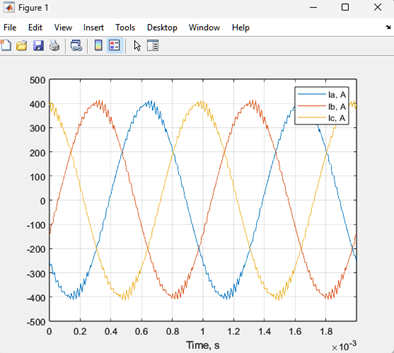
Figure 4.9. Phase-current curves obtained in the Dynamic DQ Analysis.
Configuring Dynamic FEA with PWM #
Go to the Dynamic FEA window. Be sure to tick Use initial conditions from dynamic D-Q simulation. In this case the finite-element simulation starts not from zero but from the initial magnetic field, currents, and voltages already computed in the Dynamic DQ analysis, so it reaches steady state in far fewer time steps.
For Dynamic FEA the Drive Settings are configured the same way, except that the transistor selection and the Switching dead time do not apply to Dynamic FEA.
click on image to enlarge

Figure 4.10. Dynamic FEA configured to use the initial conditions from the Dynamic DQ analysis.
click on image to enlarge
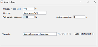
Figure 4.11. Drive Settings for the Dynamic FEA run.
On the Dynamic FE Analysis tab
- Solver type: always use Nonlinear. Linear is recommended for test purposes only.
- Simulation settings: select General. The program automatically inserts the required control script (simscript_hystpwm.m or simscript_spacevecpwm.m) depending on the PWM you chose in Drive Settings. These scripts implement the current-control algorithms (field-oriented or hysteresis) to hold the specified current and angle.
- Time step must be small compared with the PWM sampling period. If the Discretization error in Time Average Quantities in the Dynamic DQ Analysis was only a few percent, you can reuse the time step from the Dynamic DQ Analysis.
- Target RMS supply current and Target advance angle: set the desired RMS current and advance angle.
- Rotor speed dependency and Rotor speed: this example uses a fixed rotational speed.
- Save each field solution: tick this only if you need animations or cross-section distribution plots for specific time instants.
click on image to enlarge
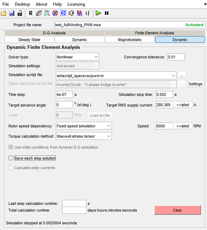
Figure 4.12. Dynamic FE Analysis settings for the PWM run.
- Click Start dynamic FE simulation.
click on image to enlarge

Figure 4.13. Running the dynamic FE simulation with PWM.
The first launch may take a few minutes to initialize. To stop the run, use Pause simulation (it finishes the current step). After the run, view the results in Time-averaged quantities and Plot Wizard.
click on image to enlarge

Figure 4.14. Time-averaged quantities and Plot Wizard buttons.
click on image to enlarge
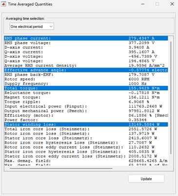
Figure 4.15. Time-averaged quantities after the Dynamic FEA (PWM) run.
As with the Dynamic DQ analysis, make sure the actual RMS phase current and Effective advance angle in Time Averaged Quantities match the Target RMS supply current and Target advance angle in the main window.
In Plot Wizard you can build a Time plot, Air gap distribution plot, cross-section distribution plot, and Animated plot. An animation or a cross-section distribution plot for arbitrary time instants can be built only if you ticked Save each field solution; otherwise only the last computed time point is available. This lets you obtain pictures of the magnetic field, the current density, or the losses during PWM commutation.
click on image to enlarge
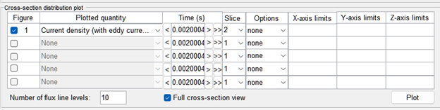
Figure 4.16. Cross-section distribution plot setup in Plot Wizard.
click on image to enlarge
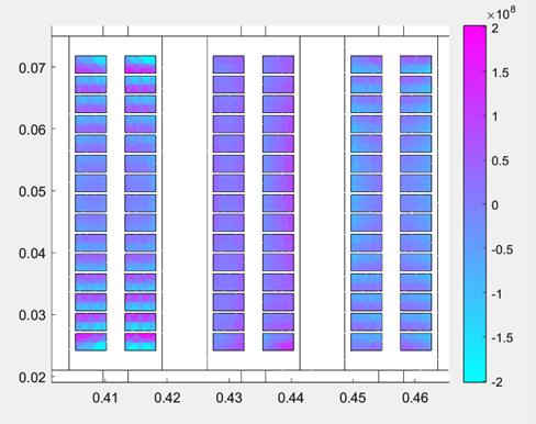
Figure 4.17. Current-density distribution in the conductors for space-vector PWM with the Full winding model.
Table 4.1 compares Dynamic FEA with the Full winding model for a sinusoidal current source supply and for space-vector PWM.
Table 4.1. Dynamic FEA (Full winding model): sinusoidal current source vs. space-vector PWM.
| Parameter | Sinusoidal current source | Space vector PWM |
| Waveform | Sinusoidal current source | Space vector PWM |
| Time step | 5e-06 s | 4e-07 s |
| Speed, rpm | 6000 | 6000 |
| Frequency, Hz | 1000 | 1000 |
| PWM sampling frequency, Hz | — | 50000 |
| Current, Arms | 280.369 | 279.4347 |
| Voltage, Vrms | 378.8457 | 377.2099 |
| Torque, Nm | 156.063 | 155.9429 |
| Stator winding loss, W | 13049.2 | 13149.5884 |
| Iron loss, W | 1770.9564 | 2551.5726 |
| Calculation time | 34 min 55 s | 5 h 33 min 34 s |
Table 4.1 shows that space-vector PWM increases the calculation time many times over. In return, accounting for the inverter and PWM reveals the extra losses from the higher harmonics: the iron losses rise by 44%, while the winding losses rise by a negligible 0.7%.
In Plot Wizard you can also plot the currents, voltages, torque, and so on.
click on image to enlarge
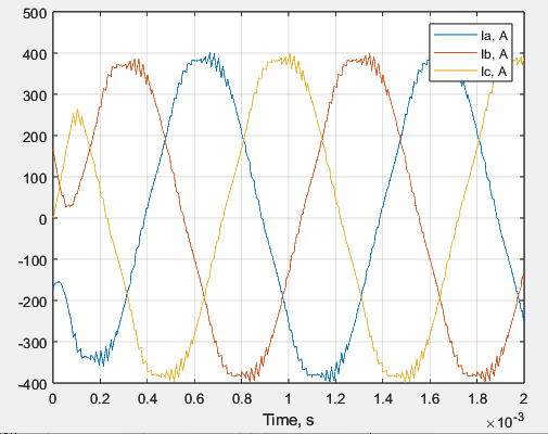
Figure 4.18. Phase-current curves.
click on image to enlarge
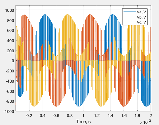
Figure 4.19. Voltages applied to the stator windings.
click on image to enlarge
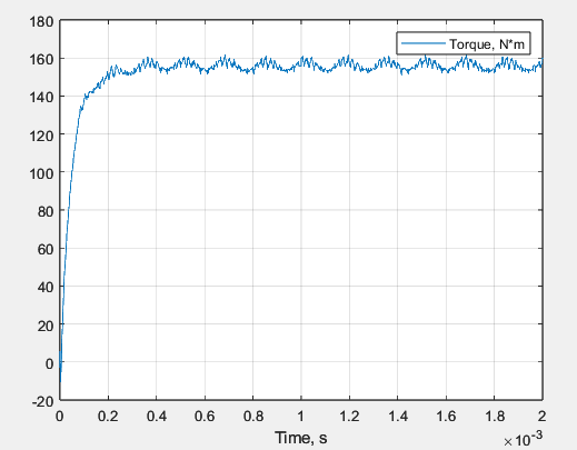
Figure 4.20. Torque curve.


