Note. The workflow described in this article applies to MotorXP-AFM 2.0 and later. In earlier versions the PCB winding representation options and the analysis workflow differ.
Before you start. This article assumes you are familiar with the Lumped and Full PCB winding models. If you are not, we recommend reading Part 1 — PCB Stator Winding Models: Lumped vs. Full first.
Introduction #
For a detailed description of the general AC-loss calculation workflow, see the AC Losses Tutorial. This article applies the same method specifically to a printed circuit board (PCB) stator.
In Dynamic Finite Element Analysis (Dynamic FEA), the current density contains two components: one produced by the external source and one induced by the changing magnetic field. The induced component includes eddy currents, the skin effect, and the proximity effect. Consequently, Dynamic FEA with the Full winding model automatically includes AC winding losses.
Magnetostatic FEA uses prescribed winding currents with an ideal sinusoidal or trapezoidal waveform and solves a sequence of static magnetic-field problems. Eddy currents do not arise in the PCB conductors, so AC winding losses are not captured.
AC losses can therefore be calculated as the difference between the stator winding loss obtained from Dynamic FEA with the Full winding model and the stator winding loss obtained from Magnetostatic FEA with the Lumped or Full winding model.
Table 2.1. Dynamic FEA vs. Magnetostatic FEA for a PCB stator.
| Aspect | Magnetostatic FEA | Dynamic FEA |
| Current density | Imposed directly and uniform in each conductor | Source-driven plus field-induced and non-uniform |
| Eddy currents (skin / proximity) | Not captured | Captured |
| AC winding losses | Excluded | Included with the Full model |
| Recommended winding model | Lumped for the fastest baseline calculation | Full for AC-loss calculation |
| Simulation time | Short | Long |
Download the example projects #
The steps and results below are based on two ready-to-open MotorXP-AFM projects. Download them to reproduce the calculation:
afm_PCB_9s12p_Lumped_winding.mxa — Magnetostatic FEA (baseline)
afm_PCB_9s12p_Full_winding.mxa — Dynamic FEA (AC losses)
Baseline losses in Magnetostatic FEA (without AC losses) #
At this stage, calculate the copper losses caused only by the active DC resistance. The current-density distribution is uniform across each conductor.
Note. Magnetostatic FEA can be run either in Design Studio (new interface) or in the main MotorXP application (legacy interface). The required input values must be identical to those used later in Dynamic FEA.
Steps in Magnetostatic FEA
- Open the PCB stator project with the Lumped winding model: afm_PCB_9s12p_Lumped_winding.mxa.
- Go to the Magnetostatic finite element analysis tab.
- In Current waveform, select Sinusoidal.
- In Current input method, select RMS supply current (or Peak supply current, or RMS current density) and enter the required value.
- Set Advance angle and Mechanical speed.
- In Simulation setup, select the required calculation accuracy. In this example, Multiple points (8 points per cogging) is used. After the run, check the Discretization error in General Results; it should not exceed a few percent.
click on image to enlarge
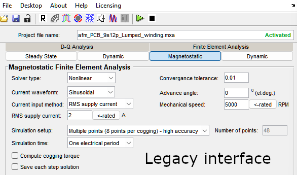
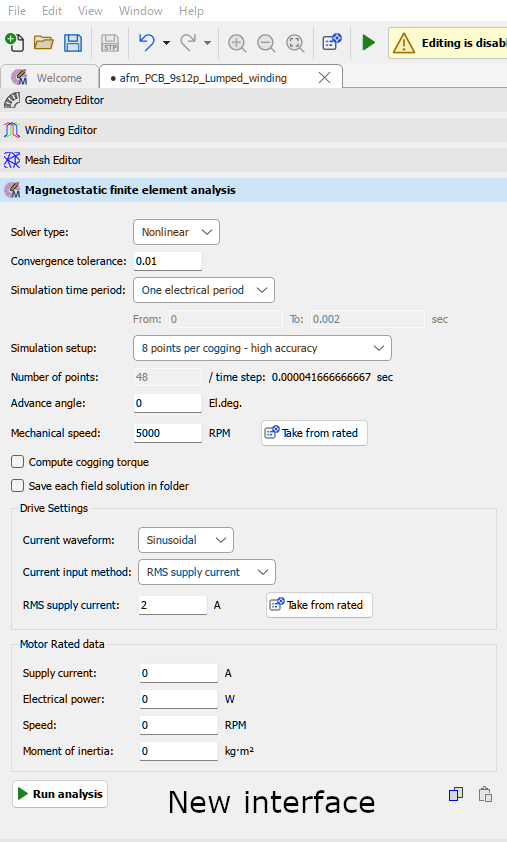
Figure 2.1. Magnetostatic FEA setup for the PCB stator: legacy MotorXP interface (left) and new Design Studio interface (right).
- Click Run analysis in Design Studio or Start magnetostatic simulation in the main MotorXP application.
- When the calculation finishes, find Stator winding loss in Results or General Results and record the value.
click on image to enlarge
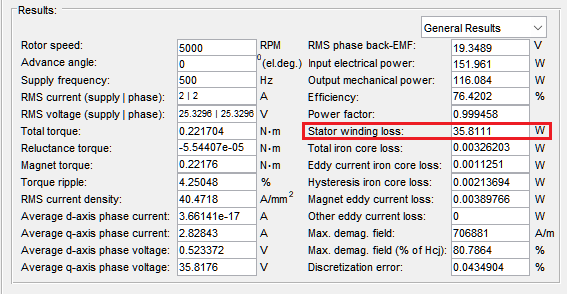
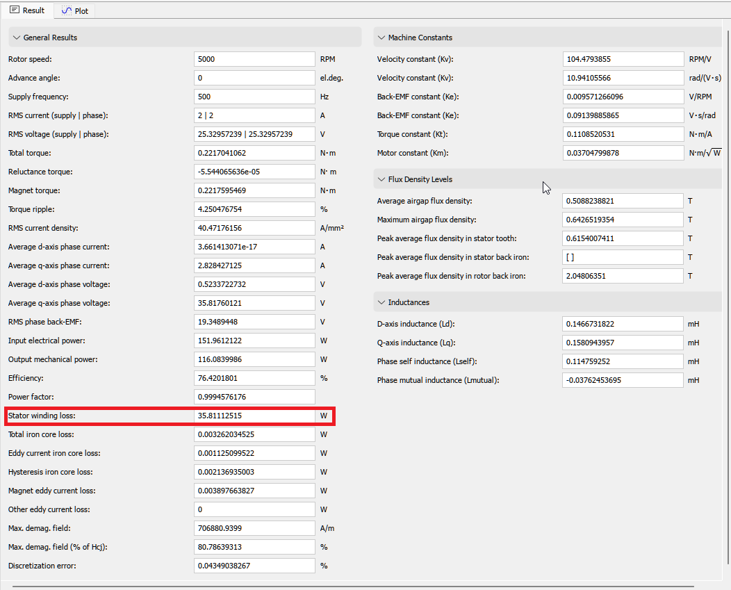
Figure 2.2. Magnetostatic FEA results: stator winding loss in the legacy MotorXP interface (left) and the new Design Studio interface (right).
- For this example, the Magnetostatic FEA stator winding loss is 35.8111 W. Save the project and do not close MotorXP.
Full losses in Dynamic FEA (with AC losses) #
Dynamic FEA calculates the total PCB copper losses, including both the losses caused by active resistance and the additional losses caused by eddy currents.
Model preparation
- Click Geometry Editor on the toolbar.
- In the stator settings, click Edit stator, find PCB geometry, and select Full.
- Set Number of turns per PCB layer, Number of PCB layers, Conductor width, Conductor height, and the other PCB parameters according to the winding data of the project.
click on image to enlarge
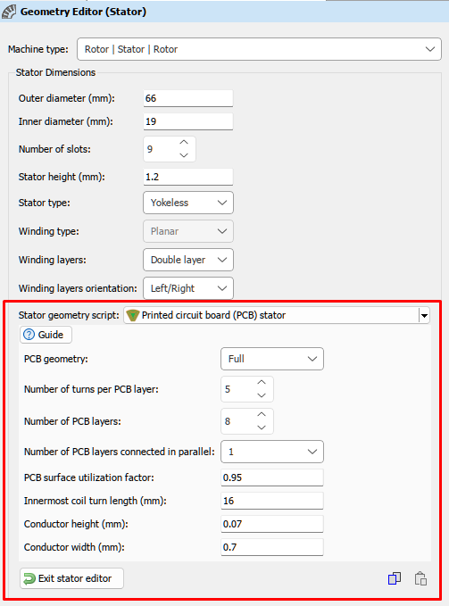
Figure 2.3. Switching the PCB stator geometry to the Full winding model.
- Open Mesh Editor. The mesh in the PCB conductor region must be sufficiently fine to capture the skin and proximity effects correctly. Avoid excessive refinement because it can substantially increase the calculation time.
- Close Design Studio and save the changes.
Steps in Dynamic FEA
- Go to the Dynamic Finite Element Analysis tab.
- In Simulation settings, select Advanced. This example uses an ideal sinusoidal current source.
- Set Stator electrical circuit file to SinCurrentSource – “3-phase current source” and click Yes when prompted. The Simulation script file changes automatically to simscript_sincurrentsource.m.
click on image to enlarge
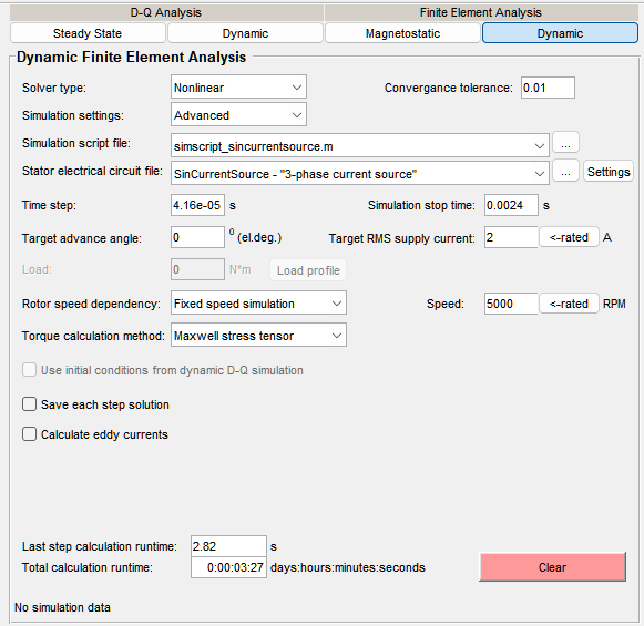
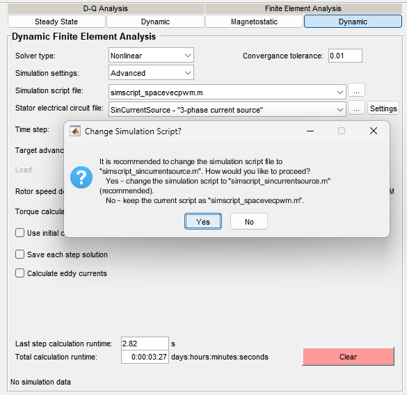
Figure 2.4. Selecting the three-phase sinusoidal current source in Dynamic FEA (left) and confirming the simulation-script change (right).
- Time step: set a sufficiently small time step. In this PCB example, the time step is 1/48 of one electrical period, matching the discretization used in Magnetostatic FEA. One electrical period is calculated as 1 / (polePairs × rpm / 60).
- Simulation stop time: set the stop time at least 20% longer than one electrical period of the supply frequency to exclude transient effects. Confirm the onset of steady state from the torque curve.
- Set Target RMS supply current, Target advance angle, and Speed to exactly the same values used in Magnetostatic FEA.
- Optional: tick Save each field solution if you want to track eddy-current changes over time or create animations and cross-section plots for individual time points.
- Click Start dynamic FEA simulation and wait for the calculation to finish.
- In the main Dynamic FEA window, click Time-averaged quantities. Average the data over 1, 2, or 3 electrical periods, or use User choice.
- Find Stator winding loss. This is the total winding loss, including the eddy-current losses.
click on image to enlarge
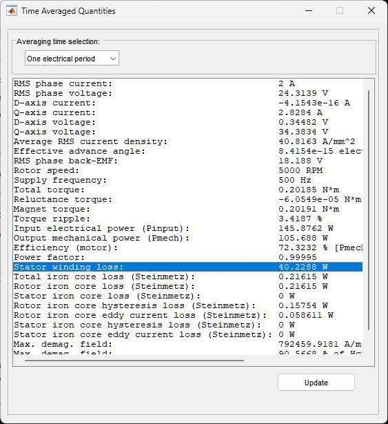
Figure 2.5. Full stator winding loss in Time Averaged Quantities.
Computing the AC losses #
Calculate the AC losses as the difference between the stator winding loss from Dynamic FEA with the Full winding model and the stator winding loss from Magnetostatic FEA:
AC losses = Pwinding (Dynamic FEA, Full) − Pwinding (Magnetostatic FEA)
Table 2.2. AC-loss calculation for the PCB stator example.
| Quantity | Value |
| Stator winding loss — Dynamic FEA (Full model) | 40.2288 W |
| Stator winding loss — Magnetostatic FEA | 35.8111 W |
| AC losses (difference) | 4.41769 W |
| AC losses as a share of total winding loss | Approximately 11% |
In this example, the additional AC losses are 4.41769 W, or approximately 11% of the total PCB stator winding loss calculated by Dynamic FEA.
Visualizing the current-density distribution #
If you ticked Save each field solution, the magnetic field, loss, and current-density data are stored for every time step, so you can view animations and the distribution pattern at each computed time point. Without it you can still view these distributions, but only for the last computed time point. Click Plot Wizard on the toolbar. In the window that opens, select Cross-section distribution plots and plot Stator current density.
click on image to enlarge
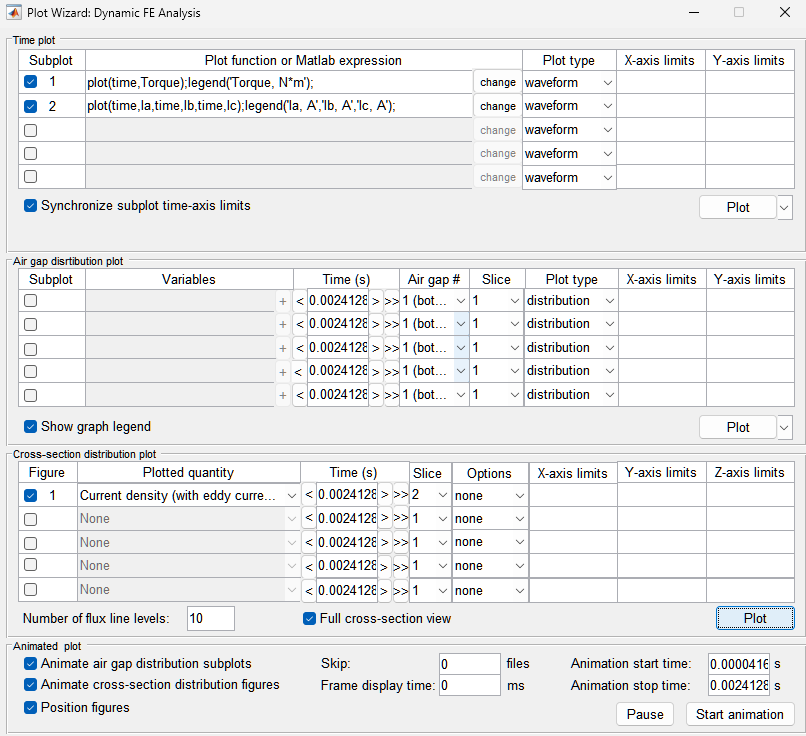
Figure 2.6. Plot Wizard: selecting the stator current-density cross-section plot.
Dynamic FEA with the Full winding model shows a non-uniform current-density distribution across the individual PCB tracks because of the skin and proximity effects. Magnetostatic FEA shows a strictly uniform current-density distribution.
click on image to enlarge
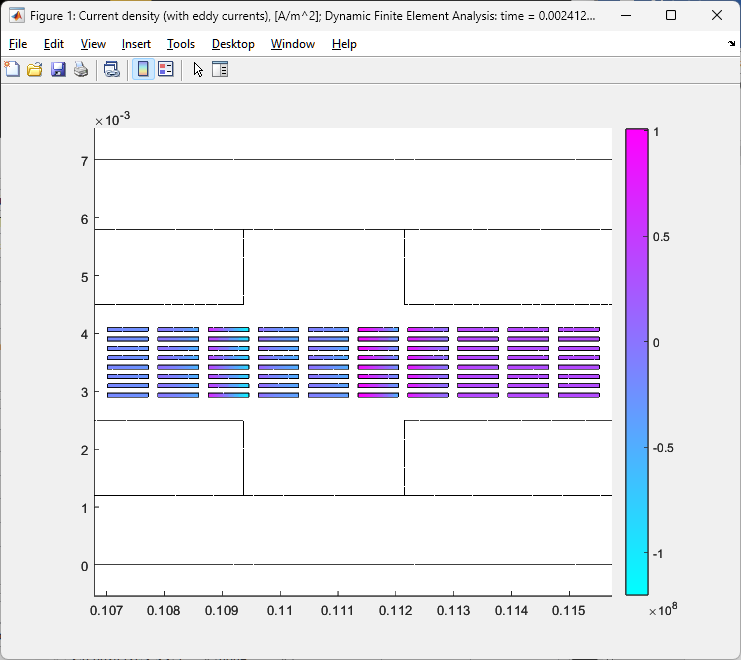
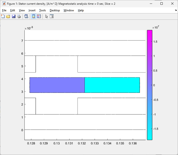
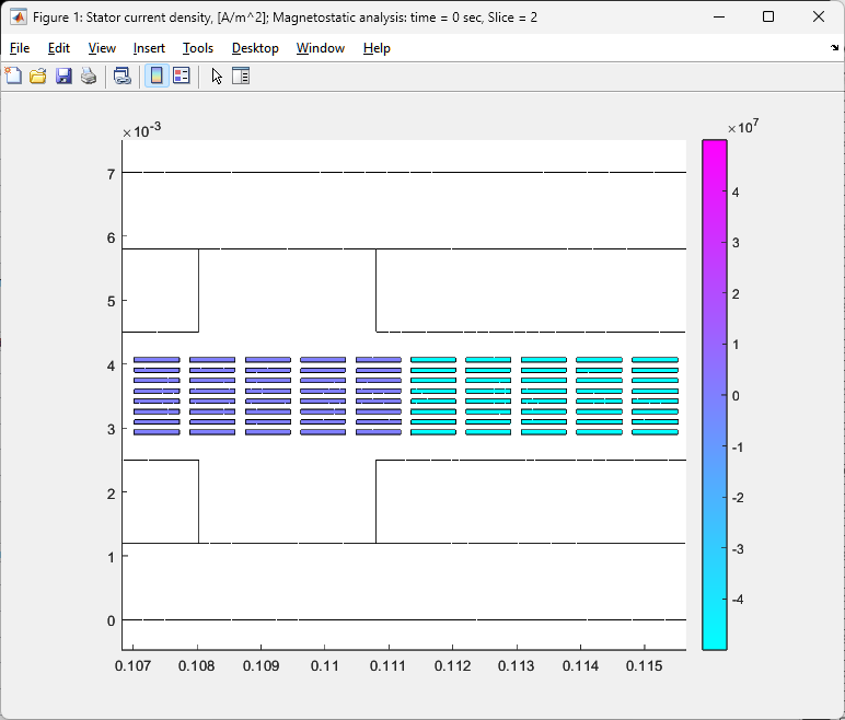
Figure 2.7. PCB stator current density: Dynamic FEA with the Full winding model (left), Magnetostatic FEA with the Lumped winding model (center), and Magnetostatic FEA with the Full winding model (right).
Note. The faceted pattern visible in the Dynamic FEA current-density plot follows the finite-element mesh. Refining the mesh in the conductor region produces a smoother and more accurate distribution, but also increases the computation time.


