Note. The workflow and comparison described in this article apply to MotorXP-AFM 2.0 and later. In earlier versions the PCB winding representation options and the analysis workflow differ.
Before you start. This article continues Part 2 — Calculating AC Losses with Dynamic FEA. We recommend reading it first.
Introduction #
This article compares four simulations of the same PCB stator project: Magnetostatic FEA with the Lumped model, Magnetostatic FEA with the Full model, Dynamic FEA with the Lumped model, and Dynamic FEA with the Full model.
All four cases use the same operating point: a rotor speed of 5000 rpm, an electrical frequency of 500 Hz, and a phase current of 2 Arms. Keeping the operating point unchanged makes it possible to isolate the effect of the analysis method and the PCB winding representation.
Magnetostatic FEA: Lumped vs. Full PCB winding model #
Table 3.1. Magnetostatic FEA: Lumped vs. Full PCB winding model.
| Parameter | Lumped | Full |
| Waveform | Sinusoidal | |
| Number of points per electrical period / time step | 48 / 4.16e-05 s | 48 / 4.16e-05 s |
| Speed, rpm | 5000 | 5000 |
| Frequency, Hz | 500 | 500 |
| Current, Arms | 2 | 2 |
| Voltage, Vrms | 25.3296 | 24.2995 |
| Torque, Nm | 0.221704 | 0.208387 |
| Stator winding loss, W | 35.8111 | 36.6569 |
| Iron loss, W | 0.00326203 | 0.00345022 |
| Calculation time | 3 min 49 s | 7 min 4 s |
In Magnetostatic FEA, the stator winding loss with the Full model is 2.36% higher than with the Lumped model because the active resistance of the Full PCB winding representation is 2.36% higher. Eddy-current losses are not captured in either Magnetostatic FEA case.
Accounting for the exact position of each conductor in the Full model can lead to a lower calculated torque compared to the Lumped model.
The Full geometry also increases the calculation time from 3 min 49 s to 7 min 4 s. For a baseline calculation without AC losses, the Lumped model is therefore the more efficient option.
Dynamic FEA: Lumped vs. Full PCB winding model #
Table 3.2. Dynamic FEA: Lumped vs. Full PCB winding model.
| Parameter | Lumped | Full |
| Waveform | Sinusoidal current source | |
| Time step | 4.16e-05 s | 4.16e-05 s |
| Speed, rpm | 5000 | 5000 |
| Frequency, Hz | 500 | 500 |
| Current, Arms | 2 | 2 |
| Voltage, Vrms | 25.3407 | 24.3139 |
| Torque, Nm | 0.22188 | 0.20185 |
| Stator winding loss, W | 35.8111 | 40.2288 |
| Iron loss, W | 0.024287 | 0.021615 |
| Calculation time | 3 min 27 s | 9 min 16 s |
Dynamic FEA with the Full model takes approximately 2.7 times longer than Dynamic FEA with the Lumped model. At the same time, the stator winding loss is 12.33% higher.
Accounting for the exact position of each conductor in the Full model can lead to a lower calculated torque compared to the Lumped model.
The difference occurs because Dynamic FEA with the Full model calculates the total PCB copper loss: the loss on the active resistance (DC losses) plus the loss caused by eddy currents (AC losses). The Full model represents every PCB track separately and therefore captures the skin and proximity effects in the conductors.
Comparison of the four cases #
Magnetostatic FEA and Dynamic FEA with the Lumped model produce practically identical stator winding losses: 35.8111 W in both cases. The Lumped representation does not resolve individual PCB tracks, so the skin and proximity effects are not captured.
Magnetostatic FEA with the Full model accounts for the change in active resistance caused by the detailed PCB geometry, but the prescribed current density remains uniform and no eddy currents arise. Only Dynamic FEA with the Full model captures the non-uniform current-density distribution and the corresponding AC winding losses.
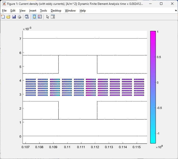
The current-density distribution over the PCB winding cross-section is compared below for all four cases.
click on image to enlarge
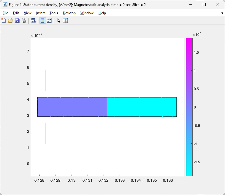
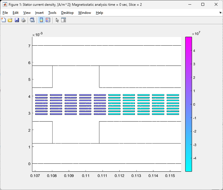
Magnetostatic FEA — Lumped (left) and Full (right)
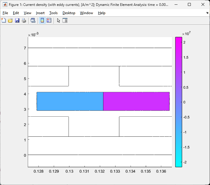
Dynamic FEA — Lumped (left) and Full (right)
Figure 3.1. Current-density distribution over the PCB winding cross-section for the four simulation cases.
In both Magnetostatic FEA cases, the current density is strictly uniform because no eddy currents arise. In Dynamic FEA with the Lumped model, the winding remains one equivalent object, so the skin and proximity effects are not resolved.
Dynamic FEA with the Full model produces a clearly non-uniform current-density distribution across the individual PCB tracks as a direct result of the skin and proximity effects. The faceted pattern visible in the plot follows the finite-element mesh.
Note. Refining the mesh in the PCB conductor region makes the current-density distribution smoother and more accurate, but also increases the calculation time.


