Note. The validation workflow and results described in this article apply to MotorXP-AFM 2.0 and later. In earlier versions the PCB winding representation options and Dynamic FEA workflow differ.
Before you start. This article continues Part 3 — Comparing Four Cases: Magnetostatic and Dynamic FEA with Lumped and Full PCB Winding Models. We recommend reading it first.
Introduction #
This article validates MotorXP-AFM Dynamic FEA with the Full PCB winding model against a full 3D model in Ansys Maxwell 3D. The comparison evaluates both calculation accuracy and computational efficiency.
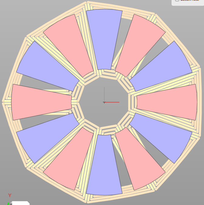
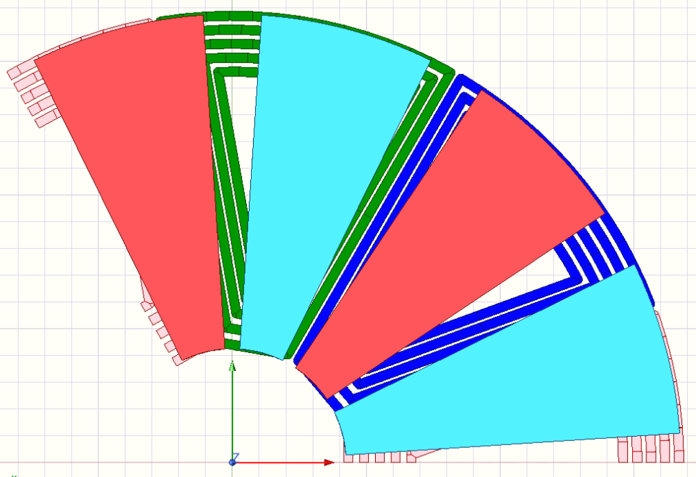
Three rotor geometries are used as validation cases (see Figure 4.1). In each row, the Ansys Maxwell 3D model is shown on the left and the corresponding MotorXP-AFM model is shown on the right. Their magnets have active radial lengths of 15 mm (initial), 20 mm (medium), and 25 mm (large). Varying the magnet length changes how much of the active PCB winding region is covered:
- 15 mm: the magnets cover only the inner, shortest part of the winding.
- 20 mm: the magnets cover the middle part of the winding.
- 25 mm: the magnets provide full radial coverage of the active winding region and its end-winding area.
click on image to enlarge
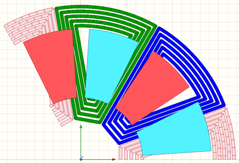
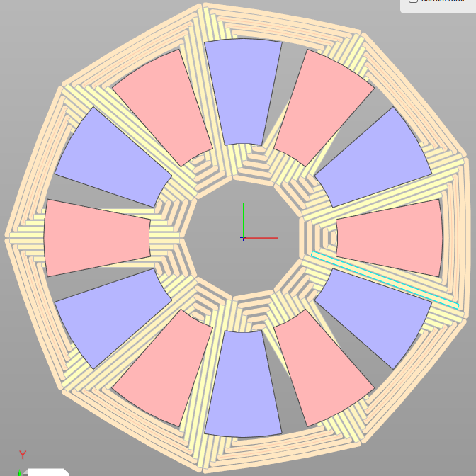
Active magnet length: 15 mm — Ansys Maxwell 3D (left) and MotorXP-AFM (right)
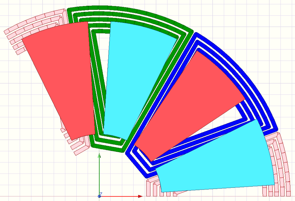
Active magnet length: 20 mm — Ansys Maxwell 3D (left) and MotorXP-AFM (right)
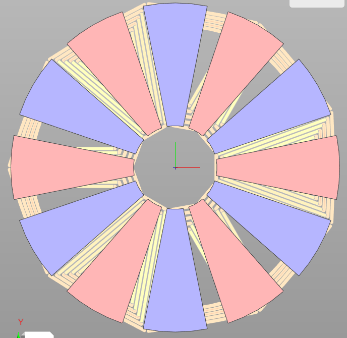
Active magnet length: 25 mm — Ansys Maxwell 3D (left) and MotorXP-AFM (right)
Figure 4.1. Rotor geometries used for validation.
Validation setup #
Figure 4.2 shows the PCB stator and magnets in Design Studio. In MotorXP-AFM, only the radial part of the winding is treated as active in the electromagnetic calculation. The end-winding part does not contribute to torque or back-EMF. Ansys Maxwell 3D uses a fully three-dimensional formulation and therefore also captures end and edge effects. This difference contributes to the remaining deviation between the two solvers.
click on image to enlarge
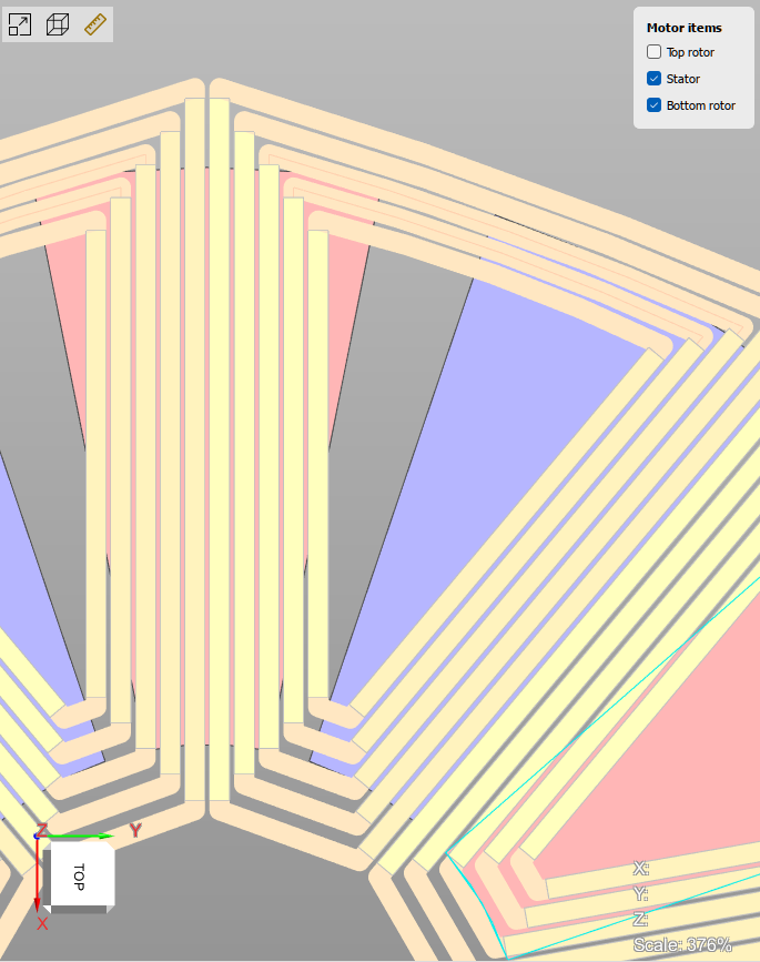
Figure 4.2. PCB stator and rotor magnets in Design Studio.
The finite-element meshes used by MotorXP-AFM and Ansys Maxwell 3D are shown in Figure 4.3. MotorXP-AFM uses a quasi-3D formulation with the PCB conductors resolved in the active slices, while Maxwell solves the complete three-dimensional geometry.
The quasi-3D formulation slices the machine with cylindrical surfaces into a set of equivalent linear machines (2D-LMMA) and solves a 2D field problem in each slice, summing the per-slice contributions to obtain the machine performance. Radial end effects are recovered by additionally solving the field in the radial cross-section and applying automatically computed geometry correction coefficients, so that the accuracy approaches a full 3D model at a fraction of the computational cost. For a detailed description of the method, see A quasi-3D finite element modelling of an axial flux machine.
click on image to enlarge
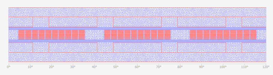
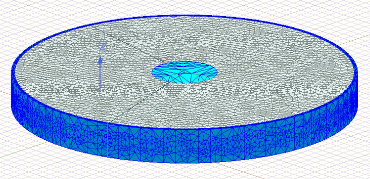
Figure 4.3. Finite-element mesh in MotorXP Design Studio (left) and Ansys Maxwell 3D (right).
Comparison results #
The tables below compare the key electromagnetic quantities and calculation time for the three configurations. The operating point is the same in every case: 5000 rpm and 2 A rms phase current. The reported difference compares MotorXP-AFM Dynamic FEA with Ansys Maxwell 3D.
Active magnet length: 15 mm #
Table 4.1. Results for the 15 mm magnets at 2 A rms.
| Parameter | MotorXP Magnetostatic |
MotorXP Dynamic FEA |
Ansys Maxwell 3D |
Dynamic FEA vs. Maxwell |
| No-load back-EMF, V rms | 18.2627 | 18.2601 | 19.2 | 5.15% |
| Torque, Nm | 0.2087 | 0.2024 | 0.2146 | 6.03% |
| Calculation time | 11 min 53 s | 15 min | 34 h 53 min | ~140× faster |
click on image to enlarge
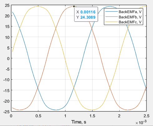
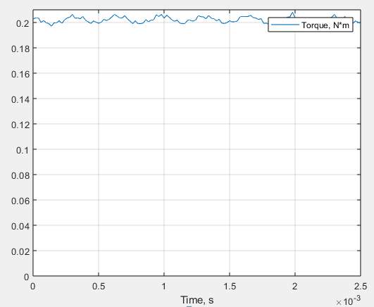
Figure 4.4. MotorXP-AFM Dynamic FEA results for the 15 mm magnets: no-load back-EMF (left) and torque (right).
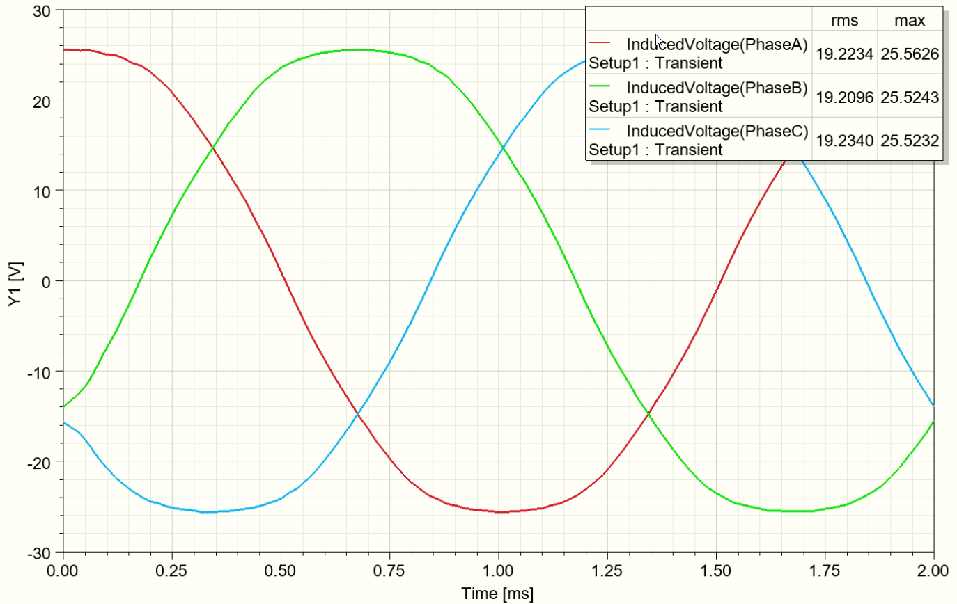
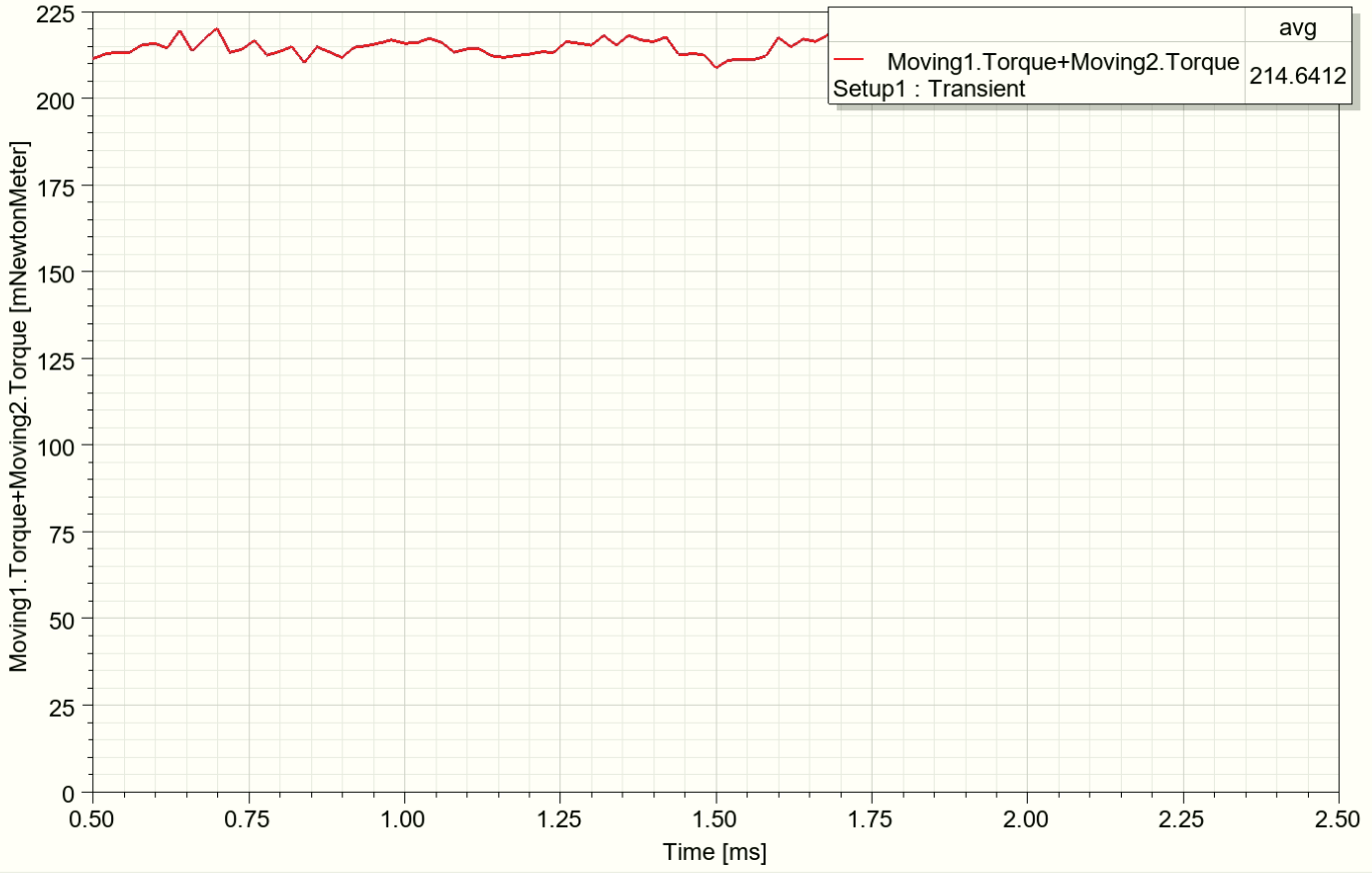
Figure 4.5. Ansys Maxwell 3D results for the 15 mm magnets: no-load back-EMF (left) and torque (right).
Active magnet length: 20 mm #
Table 4.2. Results for the 20 mm magnets at 2 A rms.
| Parameter | MotorXP Magnetostatic |
MotorXP Dynamic FEA |
Ansys Maxwell 3D |
Dynamic FEA vs. Maxwell |
| No-load back-EMF, V rms | 21.9201 | 21.9212 | 23.38 | 6.66% |
| Torque, Nm | 0.2507 | 0.2412 | 0.2529 | 4.85% |
| Calculation time | 11 min 12 s | 23 min 13 s | 33 h 20 min | ~86× faster |
click on image to enlarge
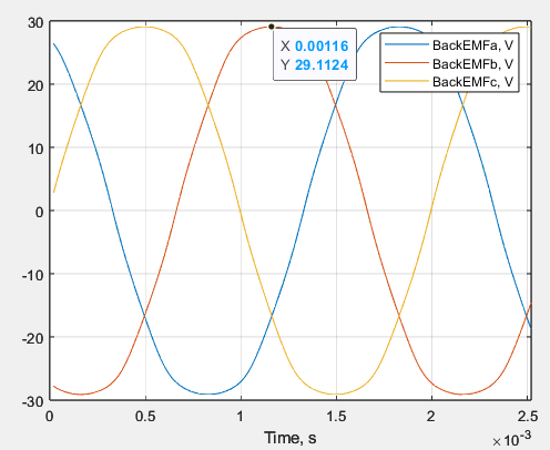
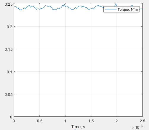
Figure 4.6. MotorXP-AFM Dynamic FEA results for the 20 mm magnets: no-load back-EMF (left) and torque (right).
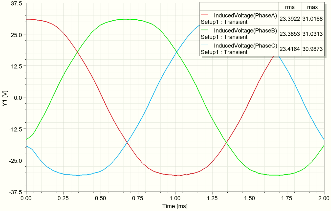
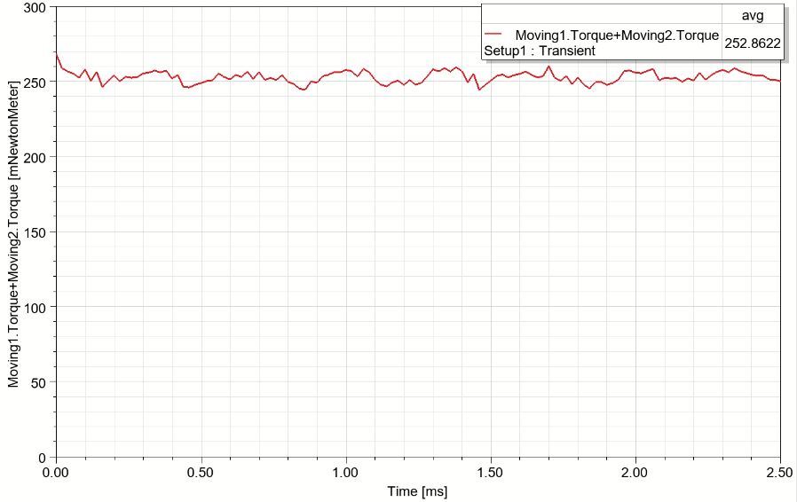
Figure 4.7. Ansys Maxwell 3D results for the 20 mm magnets: no-load back-EMF (left) and torque (right).
Active magnet length: 25 mm #
Table 4.3. Results for the 25 mm magnets at 2 A rms.
| Parameter | MotorXP Magnetostatic |
MotorXP Dynamic FEA |
Ansys Maxwell 3D |
Dynamic FEA vs. Maxwell |
| No-load back-EMF, V rms | 23.4256 | 23.4251 | 24.4 | 4.16% |
| Torque, Nm | 0.268 | 0.2577 | 0.2645 | 2.64% |
| Calculation time | 12 min 45 s | 26 min 04 s | 30 h 00 min | ~69× faster |
click on image to enlarge
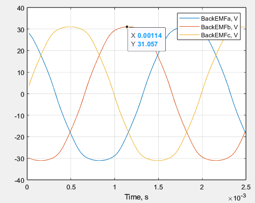
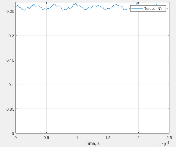
Figure 4.8. MotorXP-AFM Dynamic FEA results for the 25 mm magnets: no-load back-EMF (left) and torque (right).
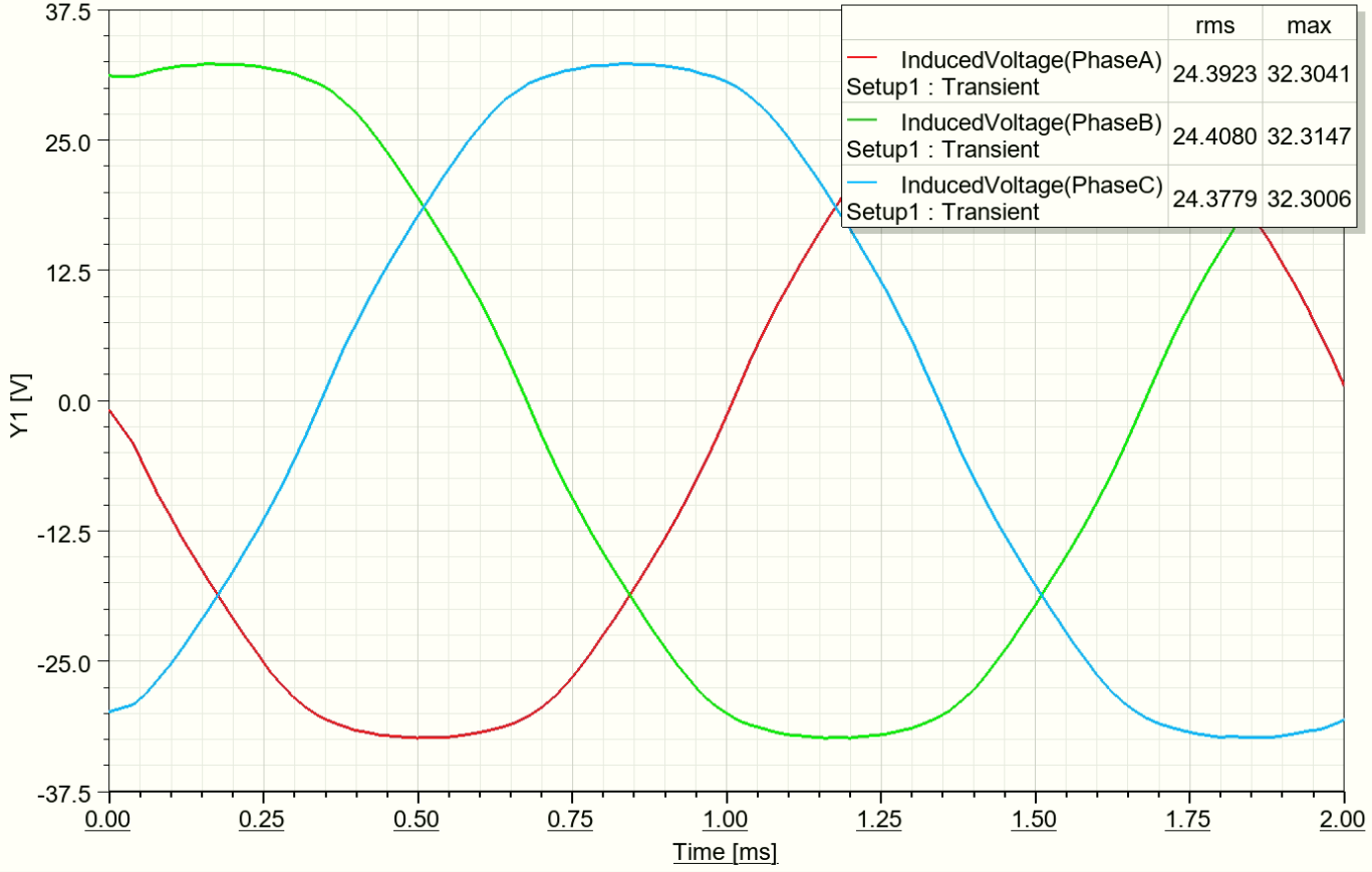
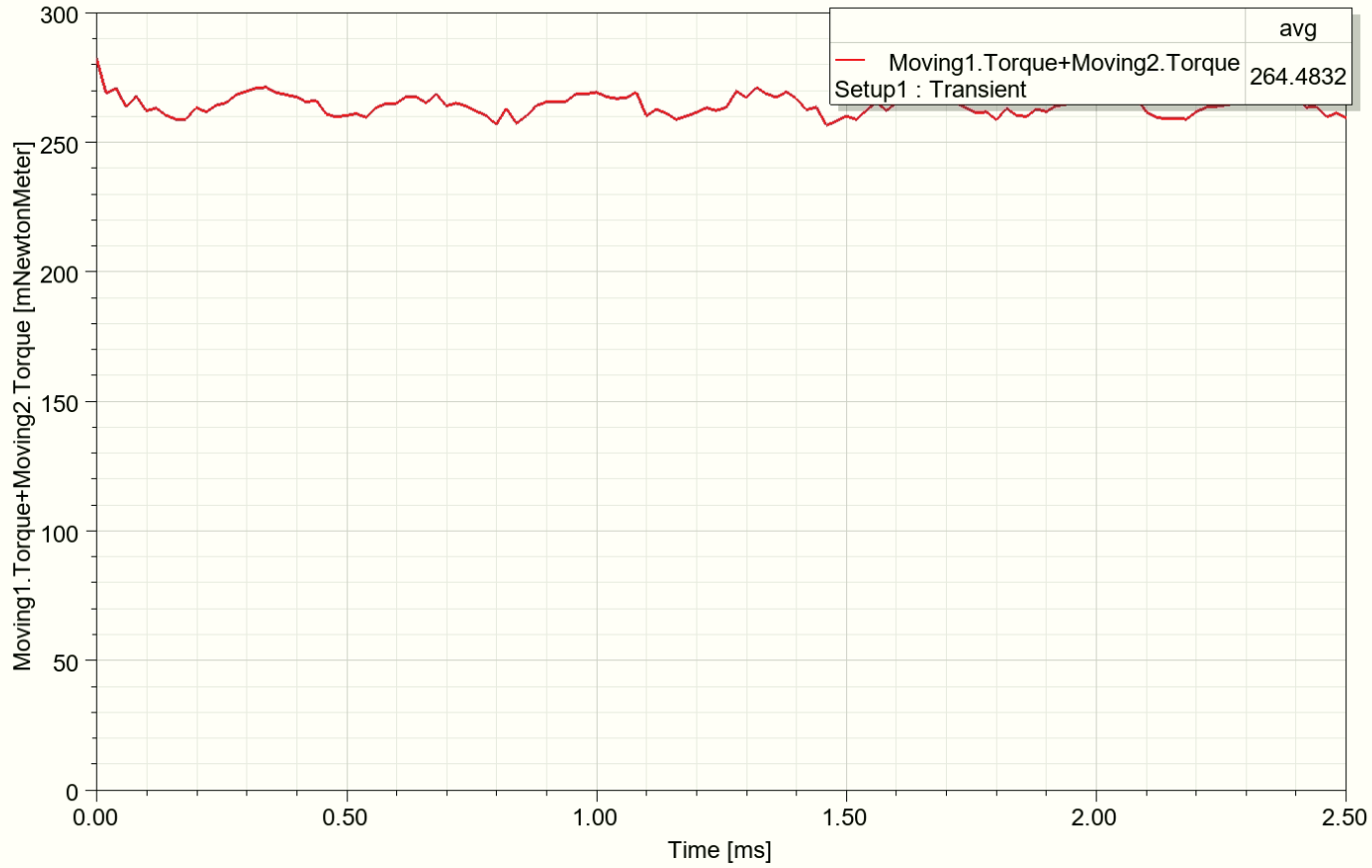
Figure 4.9. Ansys Maxwell 3D results for the 25 mm magnets: no-load back-EMF (left) and torque (right).
Accuracy and computational efficiency #
Across the three validation cases, the difference between MotorXP-AFM Dynamic FEA and Ansys Maxwell 3D remains within practical engineering limits. The no-load back-EMF difference does not exceed 6.7%, while the torque difference ranges from 2.64% to 6.03%.
As the magnet length and useful active coverage increase, the relative torque difference decreases from 6.03% to 2.64%. This indicates that the MotorXP-AFM correction factors for three-dimensional effects provide consistent results across the tested geometries.
The main advantage of MotorXP-AFM is computational efficiency. One Dynamic FEA operating point takes approximately 15 to 26 minutes, while the corresponding Ansys Maxwell 3D calculation requires approximately 30 to 35 hours. Depending on the geometry, MotorXP-AFM is approximately 69 to 140 times faster.
MotorXP-AFM is therefore well suited to active design work, parametric studies, and automatic optimization, where hundreds of geometry variants may need to be evaluated efficiently. Full 3D FEA can then be reserved for final validation of the selected design, when maximum three-dimensional fidelity is required and computational time is less critical.


