Introduction #
This tutorial shows how to prepare a model and run a transient finite element analysis that includes induced eddy currents. The example uses a Stator | Rotor | Stator machine with a yokeless rotor. This configuration is convenient for evaluating losses in both the permanent magnets and a conductive rotor component, provided that the component exists in the project and is assigned a Conductor material.
After completing the workflow, you will be able to enable or disable individual conducting regions, set their equivalent segmentation parameters, select the time step and mesh through convergence studies, and distinguish directly calculated eddy current losses from the eddy current component of electrical steel losses.
1 Where eddy currents are calculated #
Transient simulation uses the Dynamic Finite Element Analysis module, referred to below as Dynamic FEA. It solves a time-dependent electromagnetic field problem coupled to an electrical circuit. Each time step accounts for rotor rotation, nonlinear magnetic materials, and currents induced by the changing field in the selected bulk conducting regions.
Time-stepping Magnetostatic FEA can use prescribed current waveforms and estimate several loss components during postprocessing. However, it does not reproduce the feedback of induced currents on the field and circuit. Use Dynamic FEA for transients, commutation, PWM, and currents in bulk magnets or conductors.
| Component | Calculation mechanism | What to enable | Main result |
|---|---|---|---|
| Permanent magnets | Induced currents are included in the coupled field problem | Calculate eddy currents and Magnet | Magnet loss |
| Bulk rotor or stator conductor | Induced currents are included in the coupled field problem | Conductor rotor or Conductor stator | Other eddy current loss |
| Solid or SMC core | Direct field calculation is possible when required by the material and physical model | Core rotor or Core stator | Directly calculated eddy current losses in the selected region |
| Laminated core | The iron loss model calculates losses from the B waveform during postprocessing | Correct Iron material and Iron loss parameters | Piron_hyst and Piron_eddy |
Do not confuse these results. Piron_eddy is the eddy current component of the laminated iron loss model. Magnet loss and Other eddy current loss are Joule losses due to currents calculated directly in the selected conducting regions. These quantities have different physical and numerical meanings.
2 Preparing the simulation model #
2.1 SRS configuration with a yokeless rotor #
This example uses the Stator | Rotor | Stator arrangement. A yokeless rotor has no continuous ferromagnetic rotor yoke, making it convenient to observe magnet losses separately from losses in the structural conductive rotor disk. The yokeless rotor uses alternating N–S poles.


2.2 Recommended starting project #
In MotorXP-AFM, you can start with the afm_srs12_5_Lumped_winding_eddy_currents.mxa project. After opening it, check the subdomains. In the Rotor Dimensions group of Geometry Editor, Magnet carrier should be set to Conductive, and an electrically conductive material should be assigned in Materials.

The component being analyzed must exist as a separate subdomain and have the correct material type, electrical resistivity, and temperature.
3 Preparing geometry and materials #
3.1 Checking subdomain types #
Open Geometry Editor or Materials.

In DesignStudio, these correspond to the left and right areas, respectively.
Check the material type of every component in which induced currents are to be calculated.


3.2 Material properties #
| Material | Required data | Why it matters |
|---|---|---|
| Magnet | Electrical resistivity, relative magnetic permeability, magnetic properties | Resistivity directly determines induced current density and Joule losses |
| Conductor | Electrical resistivity at 20 °C, temperature coefficient, density | Resistivity is adjusted for temperature; an incorrect temperature changes the calculated losses |
| Iron, laminated | B–H curve, Iron loss coefficients, stacking factor | The field depends on B–H; Piron_hyst and Piron_eddy depend on the loss model and stacking factor |
| SMC or solid magnetic core | Electric resistivity is also required | Resistivity is used for interparticle or bulk eddy currents |
- Set the operating temperature of the materials before starting the analysis.
- Check the units of electrical resistivity in the material file.
- Do not replace an actual laminated steel stack with a solid conducting core simply to obtain a current map: that represents a different physical model.
3.3 Physical magnet segmentation #
Standard rotor geometries allow a magnet to be divided radially using Number of magnet segments in radial direction. This creates several concentric arc-shaped sections. When the segments are electrically insulated from one another, the closed current loops become smaller, which generally reduces magnet eddy current losses.

Physical condition. Segmentation reduces losses only when adjacent sections are electrically insulated. Geometric subdivision without an insulating layer should not automatically be interpreted as an interruption of the current path.
Number of magnet segments in radial direction in Geometry Editor defines the actual physical segmentation of the magnet.
4 Mesh and quasi-three-dimensional representation #
Local current densities and losses are usually more sensitive to the mesh than the integrated torque. Before running the analysis, open Mesh Editor and inspect the magnets, thin conducting components, edges, and both air gaps. Highly elongated triangles or too few elements across a thin component can produce a stable but incorrect loss integral.

| Setting | Purpose | Practical recommendation |
|---|---|---|
| Number of axial slices | Number of calculation slices in the quasi-three-dimensional model | Only one slice is supported for eddy current calculation |
| Maximum triangle side | Global upper limit on element size | Start with Auto, then reduce locally or globally for the convergence study |
| Number of layers in air gap | Field resolution across the air gap | Use a permitted odd number, typically 3, 5, 7, or 9 |
| Air gap mesh quality | Mesh density and quality in the air gap | Medium for the baseline run; High for the verification run |
| Minimum triangle angle | Limit on degenerate triangles | Increase cautiously: an excessively strict value greatly increases mesh size |
| Deflection of curve | Accuracy of curved boundary approximation | A smaller value represents arcs more accurately but increases the element count |
Pay particular attention to the element size across the magnet or conductor in the direction of the expected current gradient.
5 Enabling eddy currents in Dynamic FEA #
- In the MATLAB version of MotorXP-AFM, open the Finite Element Analysis tab and select Dynamic.
- Enable Calculate eddy currents. Open Settings next to the stator electrical circuit file. The Eddy current calculation window appears.

5.1 Eddy current calculation window #
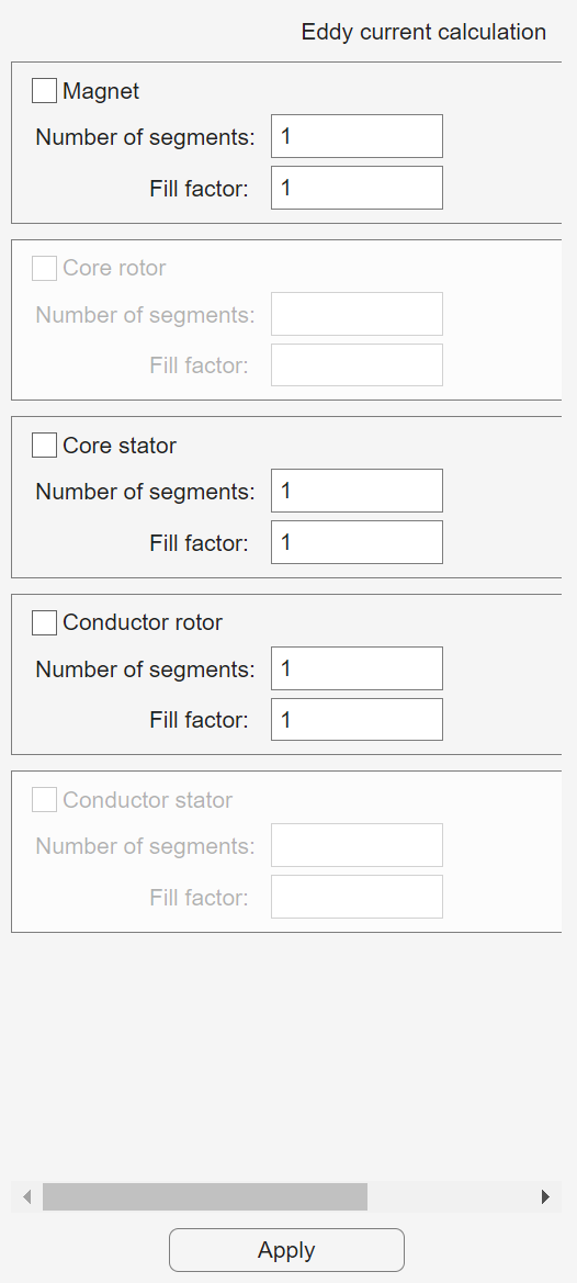
| Group | When to enable it | Comment |
|---|---|---|
| Magnet | For bulk conducting permanent magnets | The main result is reported as Magnet loss |
| Core rotor | For a physically solid or SMC rotor core | Do not enable it as a substitute for a laminated steel model |
| Core stator | For a physically solid or SMC stator core | For a conventional steel stack, use Iron loss postprocessing |
| Conductor rotor | For a disk, sleeve, retaining band, or another conductive rotor component | A Conductor subdomain must exist |
| Conductor stator | For a conductive stator component outside the standard winding | Do not duplicate ordinary phase conductors without a physical reason |
5.2 Number of segments #
This parameter sets the computational subdivision of the selected conducting group when forming the equivalent circuit of the bulk conductor. Start with the value automatically derived from the geometric subdomain. Increasing the number of segments may better resolve the spatial current distribution, but also increases the number of unknowns and the simulation time. Select the final value by checking convergence of the integrated losses.
5.3 Fill factor #
Fill factor is the effective fraction of conducting material in the quasi-three-dimensional volume under consideration. For magnets, the initial value is usually 1 or accounts for the actual coverage of the calculation segment; cores use the stacking factor; conductors use the fill factor assigned to the subdomain or 1. The value must represent the geometry and material, rather than serve as a loss-fitting coefficient.
If a group is inactive, first check for a missing subdomain or an incorrect material type. Entering Number of segments and Fill factor does not create a conducting region that is absent from the geometry.
6 Global three-dimensional eddy current setting #
Open File → Settings. In the Eddy Current Loss Calculation Settings group, locate Number of resistance layers in radial direction for calculation of 3D eddy current distribution. The default is 20 layers.

The layer count determines the radial resolution of the reconstructed three-dimensional eddy current distribution. A higher value increases detail, but also increases computational cost and data volume.
7 Dynamic FEA settings #
- Set Solver type = Nonlinear.
- Set Simulation settings = Advanced to access the electrical circuit file.
- Set Stator electrical circuit file to SinCurrentSource — “3-phase current source”. Using ideal sinusoidal current sources substantially reduces simulation time compared with PWM. For more information about PWM, see the AC Losses tutorial.

- Fill in the input fields as shown in the screenshot.

| Dynamic FEA field | Meaning | How to set it |
|---|---|---|
| Solver type | Linear or nonlinear magnetic problem | Nonlinear for an operating-point calculation with the actual B–H curve |
| Convergence tolerance | Residual tolerance of the nonlinear solver | Start with the default; reduce only when a need is confirmed, and monitor convergence at every step |
| Simulation settings | Default or custom simulation scenario and circuit | General for a standard run; Advanced for circuit/script selection |
| Simulation script file | Operating mode logic and parameter changes over time | Use the default scenario or a documented custom script |
| Stator electrical circuit file | Coupled electrical circuit | SinCurrentSource for a purely sinusoidal source; InverterCircuit for PWM |
| Time step | Time discretization interval | Choose by dividing one electrical period into a suitable number of points |
| Simulation stop time | Duration of the transient simulation | At least one electrical period plus 20% of an electrical period to allow for transient effects |
| Target advance angle | Electrical current angle | Keep the same in all compared cases |
| Target RMS supply current | Specified source or inverter current | Keep the same during a segmentation study |
| Rotor speed dependency | Prescribed or varying speed | Fixed speed for steady operation; Variable speed for acceleration or braking |
| Torque calculation method | Method used to calculate torque | Use the same method throughout the simulation series |
| Use initial conditions from dynamic D-Q simulation | Initial state from the fast D-Q model | Enable to shorten the time to steady state, for example with PWM |
| Save each step solution | Stores the field solution at every step, rather than only at the final step | Enable if field maps and animations are needed |
7.1 Choosing the time step #
For sinusoidal excitation, the fundamental electrical period can be estimated as Te = 60/(p·n), where p is the number of pole pairs and n is the speed in rpm. A practical starting point is a time step no larger than Te/100. This is not an accuracy criterion: confirm the final step by repeating the calculation with a time step half as large.
For PWM, consider the switching period and the shortest pulses. The time step must be substantially shorter than the PWM period. As an initial approximation, use 1/20 to 1/50 of the shortest relevant switching interval, then check convergence. The higher the harmonic frequency, the more sensitive the losses can be to insufficient time resolution. For more detailed PWM setup instructions, see the AC Losses tutorial.
8 Step-by-step calculation for an SRS machine with a yokeless rotor #
- Open Geometry Editor in the project.
- Make sure that the rotor is set to Yokeless and the magnets alternate N–S.
- Check the electrical resistivity of the magnets and the conductive rotor component at the operating temperature.
- Set Number of magnet segments in radial direction = 1 for the baseline case.
- Configure the mesh in Mesh Editor: use one axial slice and check the mesh resolution in the regions where eddy currents need to be calculated.
- In Dynamic FEA, enable Nonlinear, Advanced, and Calculate eddy currents.
- In Eddy current calculation, enable Magnet and Conductor rotor. For laminated stators, retain the standard Iron loss model for the stator core. Core rotor is normally not needed for a yokeless rotor.

- Accept the automatically determined Number of segments and Fill factor as the initial values. Click Apply.
- For the first run, use a sinusoidal current source, fixed speed, and the operating current. Introduce PWM after obtaining a stable baseline solution. For more detailed instructions on PWM calculations, see the AC Losses tutorial.
- Set Time step and Simulation stop time. Enable Save each step solution only if you need field maps throughout the simulation, rather than just the field map at the final step.
- Start the calculation and wait for it to finish. During the calculation, the settings window appears again to confirm eddy current calculation in the selected regions.

9 Analyzing the results #
9.1 Time Averaged Quantities #
After the calculation, select a steady-state period and record Magnet loss, Other eddy current loss, the iron loss components, average torque, and Discretization error.
The Time Averaged Quantities window summarizes electrical, mechanical, and thermal quantities over the selected interval. For eddy currents, the relevant results are Magnet loss and Rotor conductor(s) eddy current loss. For laminated cores, analyze stator/rotor iron core hysteresis loss and stator/rotor iron core eddy current loss separately.

Check Discretization error in the Time Averaged Quantities window. The recommended value is no more than 1%. If it is higher, reduce Time step first.
Discretization error represents an energy balance residual associated primarily with time discretization.
Do not average losses over the initial transient. First verify that the currents, torque, and losses have become periodic. Then select the last complete electrical period or another whole repetition interval. With a sinusoidal current source, the transient is practically absent. With PWM, reaching steady state takes appreciable time. Enabling initial conditions from Dynamic D-Q generally shortens the PWM settling time, but checking periodicity remains essential. For a more detailed analysis of PWM simulation results, see the AC Losses tutorial.
9.2 Plot Wizard #
Plot Wizard can display time waveforms, spectra, air-gap distributions, and cross-sectional maps. To evaluate eddy currents, select the available current density, magnetic flux density, and loss density quantities for the subdomain of interest. To inspect arbitrary time points and animations, the calculation must have been run with Save each step solution enabled.
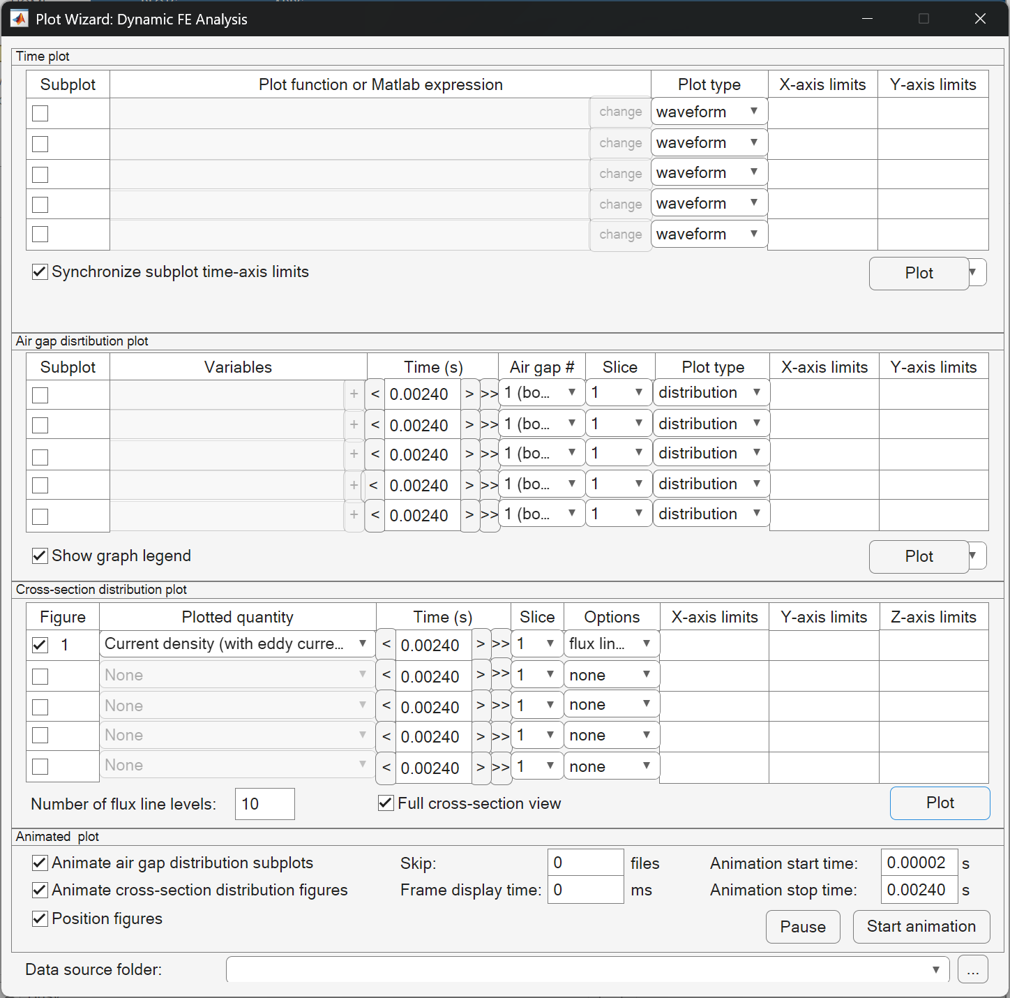

The current density maps show that the current distribution is nonuniform through the conducting material.
In this example, the current density in Conductor rotor is higher than in the magnets because the rotor conductor material has a higher electrical conductivity.
10 Evaluating eddy currents in the magnets separately #
In the eddy current settings, select only Magnet.

Run Dynamic FEA. In the Time Averaged Quantities results window, read Magnet eddy current loss.

Use Plot Wizard to display the current density distribution. The map shows that the eddy currents are also distributed nonuniformly within the magnets.


