Study Materials #
The presentation and study files below accompany the webinar AI-Assisted Axial Flux Motor Design and Optimization with MotorXP-AFM, MATLAB and AI Coding Agents. Use these materials to follow the optimization workflow and inspect the example designs.
Webinar presentation #
MATLAB scripts and MotorXP-AFM models #
Download and extract the webinar study archive. The MATLAB-files folder contains the optimization scenario scripts, evaluation functions, and saved MATLAB results. The MXA-files folder contains the baseline design, proto1.mxa, and the exported MotorXP-AFM designs.
AI-Assisted-Axial-Flux-Motor-Webinar-Materials.zip
The optimization algorithm used in this study is described in From Simulation Driven to Optimization Driven Electric Motor Design. This article focuses on AI-assisted MATLAB implementation of motor optimization, including the definition of optimization variables and two ways to handle current-density constraints.
1 Optimization Implementation Using MATLAB #
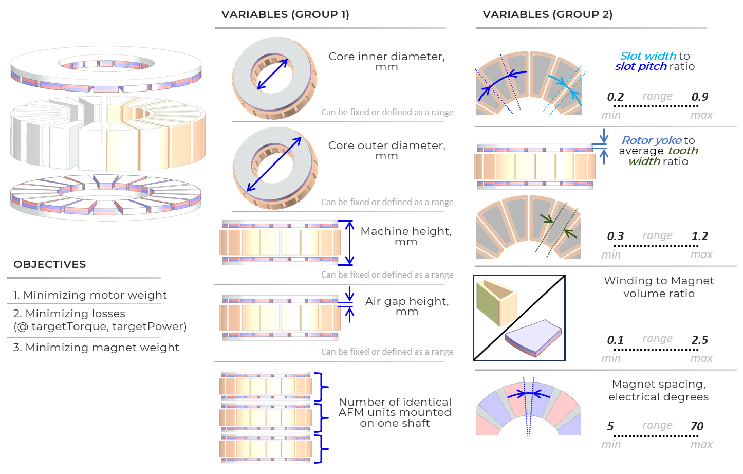
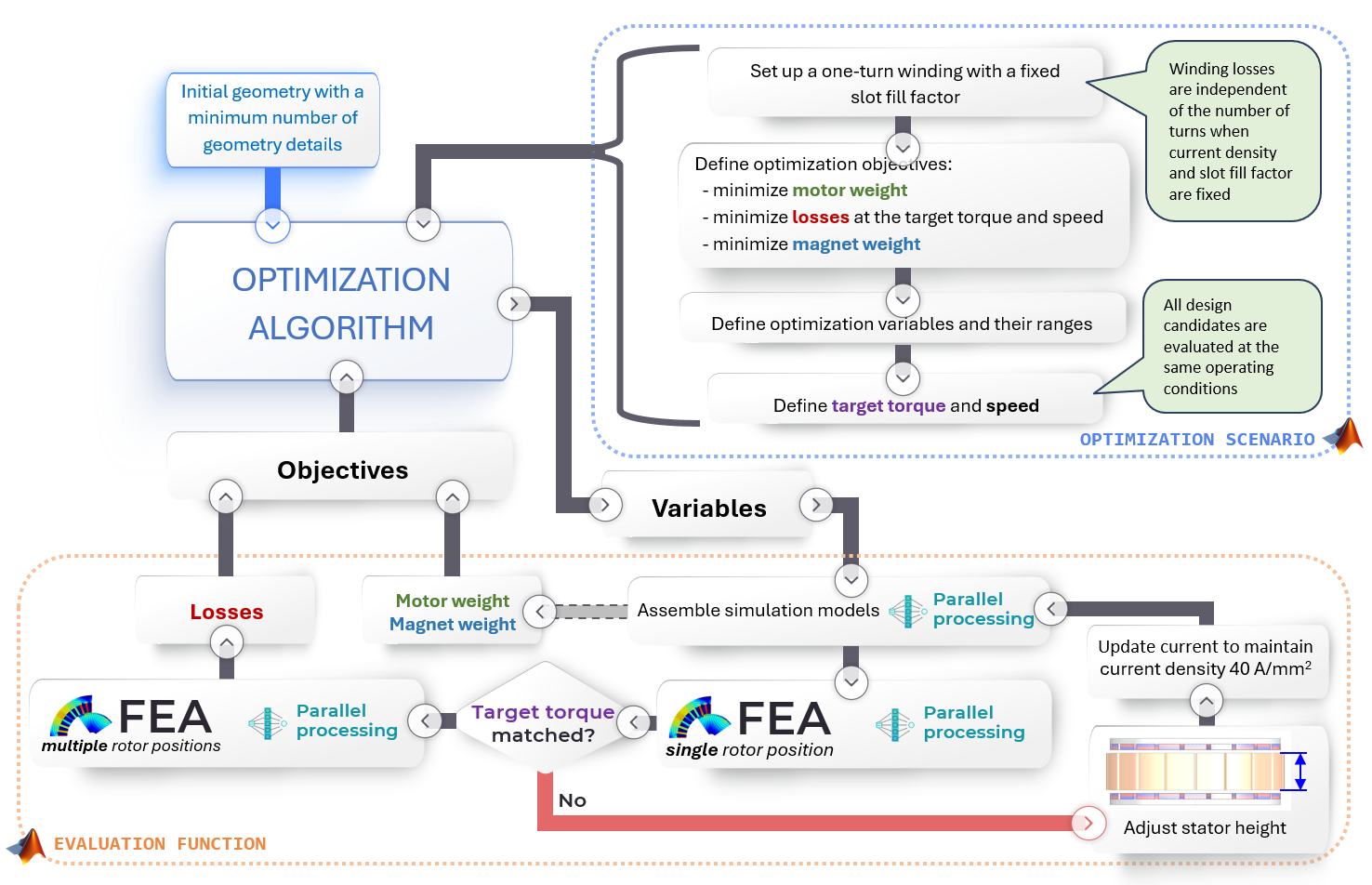
The optimization workflow uses two MATLAB files (see Figure 1):
-
The optimization scenario script defines the optimization variables, their bounds, objectives, baseline design, and calculation settings. It launches the optimizer.
-
The evaluation function receives candidate designs, updates and assembles the MotorXP-AFM simulation model, runs the required FEA calculations, and returns the objective values.
2 Optimization Variables #
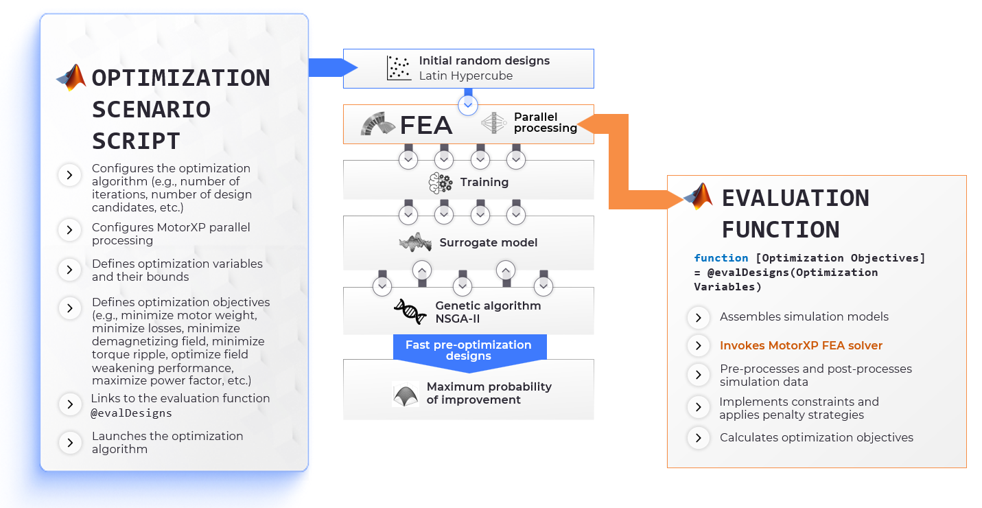
Optimization variables are defined in two ways (see Figure 2):
-
Absolute dimensions, such as the core diameters, machine height, and air gap, define the motor envelope.
-
Ratio-based and normalized parameters reflect physical relationships within the motor.
A wider slot provides more space for copper and can reduce winding resistance, but it leaves a narrower stator tooth, which may saturate. Therefore, the slot-width-to-slot-pitch ratio balances winding resistance against tooth saturation.
The rotor-yoke-height-to-average-tooth-width ratio links two parts of the same magnetic circuit. The main flux passes through both the tooth and the rotor yoke, so their dimensions should be chosen together. This ratio helps balance magnetic loading between these parts and control their relative levels of saturation.
The winding-to-magnet-volume ratio helps explore the balance between copper and magnet material. Copper volume affects winding resistance and losses, while magnet volume affects the magnetic field and magnet mass.
Magnet spacing is another normalized parameter: expressing it in electrical degrees relates it to pole pitch rather than a fixed distance. This parameter affects the air-gap flux waveform, magnetic flux leakage, and the proportion of the available rotor area occupied by magnets.
Ratio-based definitions allow similar variable ranges to be used for motors of different sizes. They also reduce geometry conflicts and exclude clearly infeasible designs before FEA. For example, defining slot width as a fraction of slot pitch, with an upper bound below one, prevents it from exceeding the available space.
The ratio-based optimization variables presented here are tailored to a rotor–stator–rotor axial-flux motor with a yokeless stator. Other axial-flux topologies may require adjustments to these variables or their definitions. An example of ratio-based optimization variables for a radial-flux motor is provided in AI-powered electric motor design.
3 Optimization Scenario and Evaluation Function Implementation #
The optimization is implemented through two MATLAB files: an optimization scenario script and an evaluation function (see Figure 3).
-
The optimization scenario script defines the optimization variables and their ranges, the objectives, and the calculation settings, including parallel processing. It then launches the optimization algorithm, which passes candidate designs to the evaluation function as vectors of variable values.
-
The evaluation function converts each candidate into a MotorXP-AFM simulation model, checks its geometry, runs the required calculations, and returns the objective values.
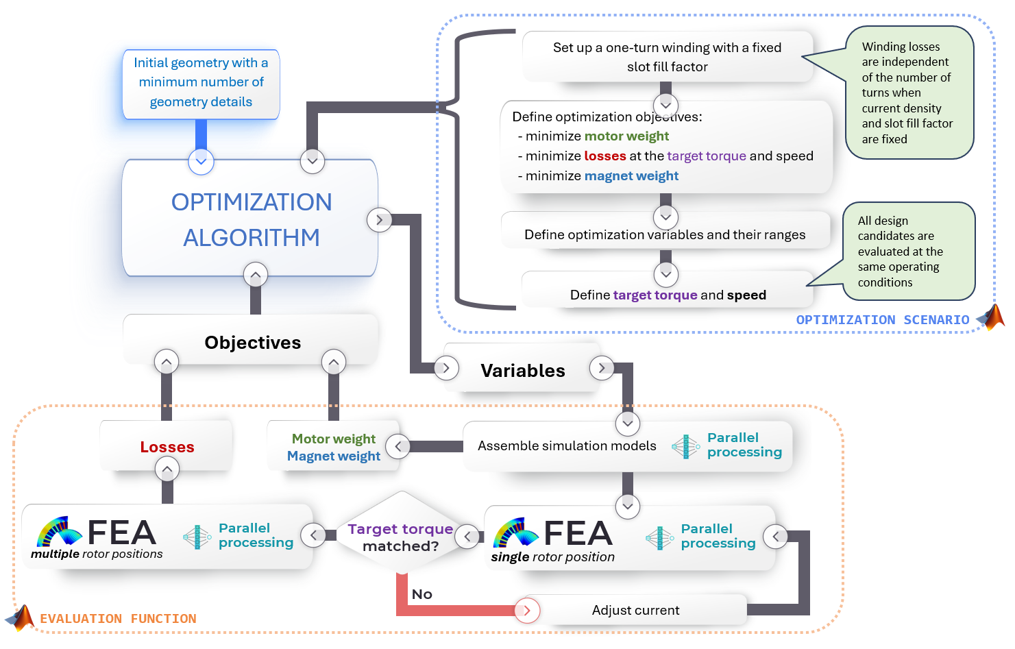
The evaluation function processes each candidate through the following steps:
-
Convert variables and validate geometry. The evaluation function converts the candidate values into MotorXP-AFM parameters and calculates the dependent dimensions. It checks that the geometry is valid and fits within the specified dimensional limits before assembling the simulation model. Candidates with incompatible dimensions are rejected before FEA, avoiding unnecessary calculations.
-
Assemble the winding model. The study uses a one-turn lumped winding model with a fixed slot fill factor. For the same geometry, current density, and slot fill factor, the calculated DC winding loss is independent of the number of turns. This allows the geometry to be optimized before selecting the final number of turns to match the voltage and current requirements.
-
Match the target operating point. All candidates are evaluated at the same target torque and speed. After assembling a model, the evaluation function adjusts the current and repeats the torque calculation until the target torque is reached within the specified tolerance. This iterative adjustment accounts for magnetic saturation, which can make the relationship between current and torque nonlinear.
-
Calculate and return the objectives. The final FEA results provide the electromagnetic losses at the target operating point, while motor mass and magnet mass are calculated from the geometry and materials. The evaluation function applies the selected current-density constraint strategy and returns the three objective values to the optimization algorithm.
Model assembly and FEA can run in parallel for several candidates to reduce the overall calculation time.
4 AI Coding Agents in the Optimization Workflow #
Many motor design engineers prefer to focus on engineering and motor physics rather than writing and debugging code. Automated optimization, however, requires MATLAB scripts that translate the design requirements into a working study. AI coding agents can handle much of this programming work, allowing the engineer to concentrate on the optimization strategy and the results.
AI coding agents, such as OpenAI Codex (ChatGPT) and Claude Code, create and modify the optimization scenario and evaluation function while the motor design engineer oversees the overall process (see Figure 4). The agent can propose variables, objectives, constraints, and practical ranges, map variables to MotorXP properties, implement geometry checks, and prepare validation scripts.

The collaboration follows these steps:
-
Request an implementation proposal. Ask the agent to explain the proposed implementation before creating any files.
-
Review and approve the strategy. The engineer reviews the objectives, constraint handling, variable bounds, and calculation settings.
-
Generate the MATLAB files. After approval, the agent generates the optimization scenario and evaluation function.
-
Test and correct the code. If a test run produces an error, the engineer can provide the exact MATLAB error message and ask the agent to correct the code.
-
Validate the optimized design. The engineer makes the final decisions on the optimization strategy and validates the optimized design.
MotorXP skills for AI coding agents are available in MotorXP AI Tools.
5 First Study Task Statement #
The first prompt gives the agent the complete engineering contract: topology, dimensions, operating point, current-density limit, materials, optimization objectives, and the optimization run settings. It asks for a proposed strategy based on the baseline MotorXP-AFM design (proto1.mxa, available in the Study Materials) but explicitly prohibits creating MATLAB files before approval.
Terms highlighted in yellow are explained in Notes on highlighted terms immediately below Prompt 1. These notes provide guidance and are not part of the prompt.
Geometry and manufacturing constraints:
- AFM topology: rotor-stator-rotor with yokeless stator
- Fixed outer diameter: 49.5 mm
- Fixed air gap: 1.3 mm
- Motor length <= 20 mm
- Slot fill factor: 0.35
- Magnet segmentation: radial, 4 segments

Operating point and electrical loading:
- Torque: 0.5 Nm
- Speed: 3200 RPM
- Current density <= 40 A/mm²

Materials:
- Magnet: N48SH
- Stator core: M-19 29 Ga
- Rotor core: 1010
- Winding: Copper

Temperatures:
- Winding: 40° C
- Magnet: 30° C

Selected slot/pole configuration:
18 slots, 20 poles

Optimization objectives:
Minimize motor weight, total losses (@ 0.5 Nm and 3200 RPM), and magnet weight.

Suggest an optimization strategy for the above specifications and requirements based on the generalized normalized-variable optimization scenario, including:
- Optimization variables and their ranges
- Penalty function: Apply a penalty proportional to the amount by which the current density exceeds 40 A/mm²
- Optimization objectives
- Optimization algorithm and parallel processing settings

Use the following optimization run settings:
Initial dataset: 100 designs
Sequential batch size: 12
Iterations: 50
Total evaluations: 100 + 50×12 = 700

Use "[local computer path]\SimFiles\Webinar_Sept2026\proto1.mxa" as the baseline design.
Extract the optimization variable values from the baseline design and suggest appropriate variable ranges based on the baseline values and the geometry constraints.
Use the baseline design as a reference point on the Pareto plot for comparison and assessment of the improvements.
Do not create any M-files before receiving approval.
Notes on highlighted terms #
Penalty function is one way to handle optimization constraints. If a candidate design requires a current density above 40 A/mm², its objective values are increased proportionally to the constraint violation, making the design less favorable and steering the optimizer toward the feasible design region.
[local computer path]. Replace this placeholder with the actual path on your local computer.
After reviewing and approving the agent’s proposed logic, use the following prompt to generate the corresponding MATLAB files (see Prompt 2).
Use the suggested settings, ranges, and parameters.
Create the optimization scenario and evaluation function M-files in "[local computer path]\CustomScripts\Webinar_Sept2026"
If possible, do not create more than two M-files for this optimization study.
The prompts above can be copied and adapted to other studies.
6 Current Density Constraint Using a Penalty Function #
In the first study, current density is not fixed at a single value. For each candidate design, the evaluation function adjusts the current until the motor produces the target torque. It then calculates the corresponding winding current density and compares it with the limit of 40 A/mm².
The objective values returned to the optimizer depend on whether the candidate satisfies this limit:
-
Current density is within the limit. The evaluation function returns the calculated motor mass, total losses, and magnet mass without modification.
-
Current density exceeds the limit. The evaluation function increases the objective values returned to the optimizer in proportion to the constraint violation. This increase implements the penalty: the physical results remain unchanged, but the optimizer receives higher objective values. Since the optimizer minimizes these objectives, the penalty makes the candidate less attractive and encourages the search toward designs that satisfy the current-density constraint.
One way to implement this is to calculate the relative constraint violation and use it to scale the objectives:
violation = max(0, (Jrequired - Jlimit) / Jlimit);
penaltyFactor = 1 + penaltyCoefficient * violation;
penalizedObjective = rawObjective * penaltyFactor;
In this formulation:
-
Jrequired is the current density needed to reach the target torque.
-
Jlimit is the permitted maximum current density.
-
max(0, …) ensures that designs within the limit receive no penalty.
-
penaltyCoefficient controls how strongly the optimizer is discouraged from selecting designs that exceed the limit.
Example. A current density of 44 A/mm² exceeds the 40 A/mm² limit by 10%. With a penalty coefficient of 2, the penalty factor is 1.2, so each objective value returned to the optimizer increases by 20%. This changes how the optimizer ranks the candidate, but it does not change the motor’s actual mass or calculated losses.
The physical results and penalized objective values should be stored separately. Use the physical results to compare motor performance, and check constraint compliance explicitly when selecting the final design. A penalty discourages constraint violations but does not guarantee that every design produced by the optimization satisfies the limit.
7 Fixed Current Density Inside the Evaluation Function #
In the second study, the evaluation function implements the current-density constraint directly by adjusting the motor geometry. Every accepted candidate must produce the target torque at a fixed current density of 40 A/mm². To meet both requirements, stator height becomes a dependent dimension calculated inside the evaluation function (see Figure 5).
For each candidate, the evaluation function performs the following steps:
-
Set a trial stator height. Calculate the available winding cross-sectional area.
-
Set the current and calculate torque. Set the current to maintain a current density of 40 A/mm² and run FEA to determine the torque.
-
Adjust the stator height. If the torque is below the target, increase the stator height. If it is above the target, reduce the height. After each adjustment, recalculate the winding area and current before the next FEA calculation.
-
Repeat until the target torque is reached. Keep the search within the permitted dimensional bounds and continue until the calculated torque matches the target within the specified tolerance.
This process requires an iterative search because torque may not change in direct proportion to stator height. Magnetic saturation, particularly in the stator teeth, can make the relationship nonlinear.
The evaluation function also checks the total motor length. If the target torque cannot be reached at the fixed current density without exceeding the 20 mm length limit, the candidate is rejected. Accepted candidates therefore satisfy both the target-torque requirement and the fixed-current-density condition within the defined tolerances. Their final stator height is stored with the results and used when the selected design is exported to an MXA file.
For this formulation, the winding-to-magnet-volume ratio is replaced with absolute magnet height as an optimization variable. Adjusting stator height changes winding volume. Retaining the volume ratio would therefore require magnet dimensions to change during the same adjustment. Using absolute magnet height keeps the magnet geometry fixed during the stator-height search and makes the constraint implementation simpler.
8 Fixed Current Density Task Statement #
The next prompt asks the agent to retain the first study’s settings where possible, but change the constraint implementation and the variable used for magnet height. As before, it requests a proposal before any MATLAB files are written.
For the same study, suggest an optimization strategy with the current density fixed at 40 A/mm²:

- Where possible, use the same optimization variables and ranges.
- Minimize motor weight, total losses at 0.5 Nm and 3,200 rpm, and magnet weight.
- To maintain the fixed current density, adjust the stator height until the target torque is matched. Note that, due to stator tooth saturation, torque may not be linearly proportional to stator height.
- Replace the winding-to-magnet volume ratio with the absolute magnet height. This will simplify the dependent-height formulation.
- Use the same optimization algorithm and parallel-processing settings.

Use the same file, "[local computer path]\SimFiles\Webinar_Sept2026\proto1.mxa", as the baseline design.
Use the baseline design as a reference point on the Pareto plot for comparison and assessment of the improvements.
Do not create any M-files before receiving approval.
After reviewing and approving the proposed strategy, use the following prompt to generate the optimization scenario and evaluation function MATLAB files.
Use the suggested settings, ranges, and parameters.
Create the optimization scenario and evaluation function M-files in "[local computer path]\CustomScripts\Webinar_Sept2026"
If possible, do not create more than two M-files for this optimization study.
9 Comparison of the Two Constraint Methods #
The two constraint methods guide the optimization toward different combinations of motor mass and losses (see Figure 6).
-
Current-density constraint using a penalty function. In the first study, current density varies between designs according to the current needed to produce the target torque. Candidates within the 40 A/mm² limit receive no penalty, while candidates above it become less attractive to the optimizer. This allows the study to explore designs with lower electrical loading, which may reduce losses at the expense of greater motor mass.
-
Fixed current density with dependent stator height. In the second study, every accepted candidate operates at 40 A/mm², and stator height is adjusted to meet the target torque. In this example, the resulting designs are concentrated in a smaller region of the mass-loss plot. The study includes low-mass designs with high power density, but it does not reach the same low-loss region as the first study.
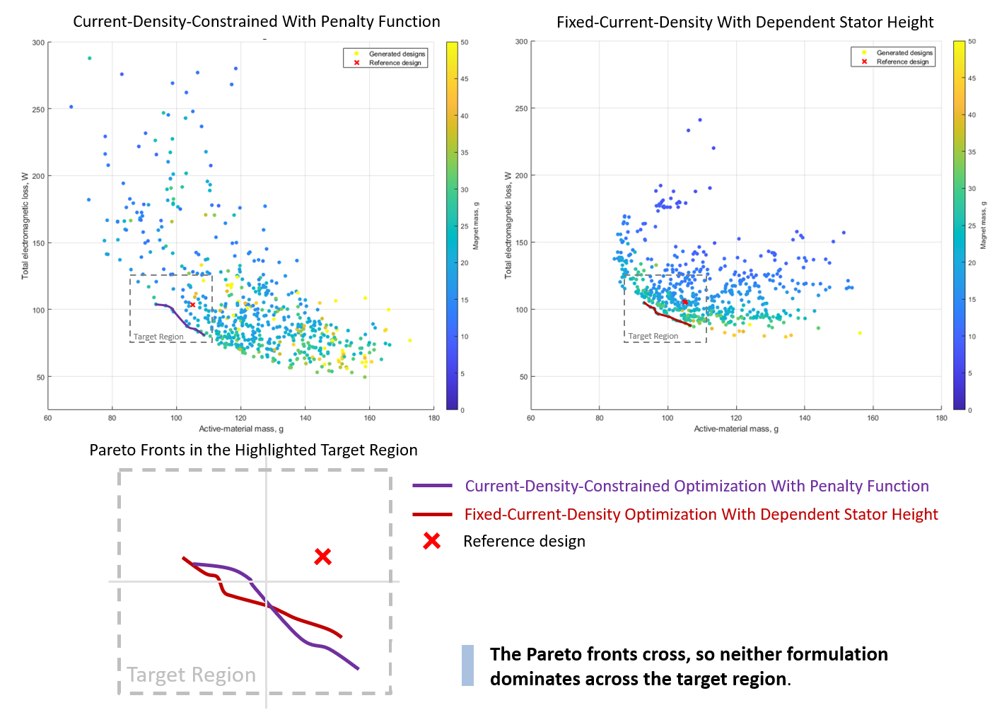
Within the highlighted target region, the Pareto fronts cross. For some mass values, the first study provides lower losses; for others, the second study provides a better trade-off. Neither formulation gives better results throughout the entire region shown.
The preferred design therefore depends on the required balance between mass and losses, with magnet mass also considered as the third objective. This comparison shows how the choice of constraint implementation can influence the optimization results.
10 Focused Optimization Study #
The first two studies identify a promising region of the design space, but relatively few evaluated designs lie close to the required mass and loss values. A focused study concentrates additional calculations in this region by narrowing the optimization-variable ranges around selected designs from both studies. Small margins around the selected values allow the optimizer to explore nearby alternatives.
The initial and focused variable ranges are compared in Table 1. Based on these ranges, the focused search volume is approximately 7.0% of the original search volume.
| Variable | Definition | Initial range | Focused range | Width reduction |
|---|---|---|---|---|
| x1 | Slot-width angle / slot-pitch angle | 0.550–0.880 | 0.590–0.740 | 54.5% |
| x2 | Rotor-yoke height / tooth width | 0.450–1.150 | 0.450–0.750 | 57.1% |
| x3 | Equivalent winding/magnet volume, K | 0.200–1.200 | 0.400–1.200 | 20.0% |
| x4 | Magnet spacing [electrical degrees] | 10–55 | 10–50 | 11.1% |
| x5 | Total motor length [mm] | 12–20 | 14.5–20.0 | 31.3% |
| x6 | Inner diameter / outer diameter | 0.500–0.750 | 0.565–0.750 | 26.0% |
Use the following prompt to request a focused optimization strategy based on selected designs from both previous studies. The selected designs are shown on the Pareto plots (see Figure 7).
Attach Figure 7 when submitting Prompt 5 so the agent can identify the selected designs. Download Figure 7.
Prepare a focused optimization study based on two previous optimization studies: Current-Density-Constrained Optimization with Penalty Function and Fixed-Current-Density Optimization with Dependent Stator Height.
- Use the optimization variables from the first study (Current-Density-Constrained Optimization with Penalty Function).
- For design candidates with current density no greater than 40 A/mm², perform the optimization without additional adjustment. For design candidates with current density above 40 A/mm², increase the stator height as needed to maintain a fixed current density of 40 A/mm², using the same approach as in the Fixed-Current-Density Optimization with Dependent Stator Height.
- Extract the optimization-variable values for the designs selected on the attached Pareto plots from both optimization studies. Based on the extracted values, propose focused variable ranges with small margins around the selected designs. Note that some of the selected designs are not nondominated.
- For each extracted design, show its position within the proposed variable ranges and report its objective values for verification.
- Use the extracted designs as deterministic seed points in the initial surrogate-model training dataset, together with the remaining LHC-generated initial designs.
- Use the baseline design as a reference point on the Pareto plot for comparison and assessment of the improvements.

Do not create any M-files before receiving approval.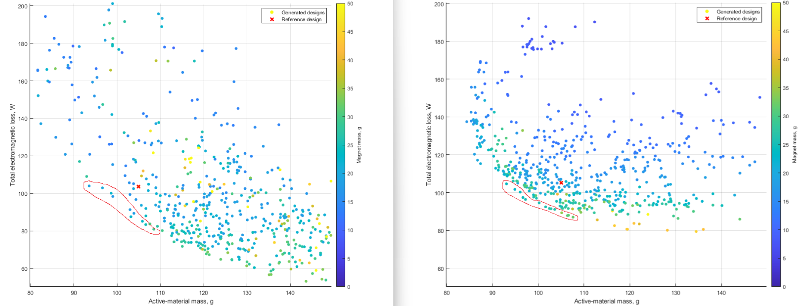
The selected designs are used as deterministic seed points in the initial dataset. These seeds give the study known starting points near the region of interest. The remaining initial candidates are generated using Latin hypercube sampling within the reduced ranges.
Some selected seeds may be dominated by other designs, but they can still provide useful information about nearby parts of the design space. All seeds and newly sampled candidates must be assessed consistently under the focused study’s evaluation rules.
The focused study combines variable current density from the first study with the stator-height adjustment used in the second:
-
Current density is no greater than 40 A/mm². If a candidate produces the target torque within this limit, its stator height remains unchanged.
-
Current density exceeds 40 A/mm². The evaluation function increases stator height and recalculates the current until the target torque is reached at 40 A/mm² within the specified tolerances. Candidates that cannot satisfy these requirements within the dimensional limits are rejected.
This approach retains designs that already meet the current-density limit while adjusting other candidates through a dependent geometry change. Together with the narrower ranges and selected seeds, it concentrates the available calculations on finding additional feasible trade-offs near the design requirements.
11 Focused Study Results #
The narrower variable ranges and the use of promising designs from the previous studies produce a more densely populated Pareto front in the target mass–loss region (see Figure 8). This provides more candidates close to the design requirements and makes it easier to compare the available trade-offs.
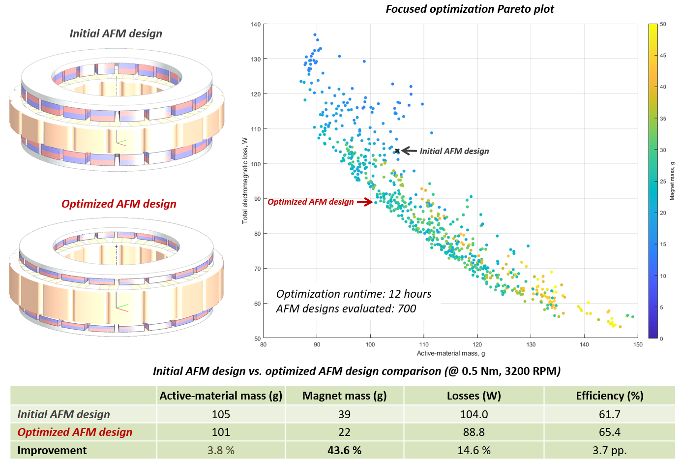
Compared with the baseline, the selected design achieves:
-
Nearly the same active-material mass.
-
Approximately 44% less magnet material.
-
About 15% lower electromagnetic losses.
-
An efficiency increase of 3.7 percentage points at the target operating point.
The selected design (design_f1=100.9939_f2=88.7692.mxa, available in the Study Materials) is exported from the Pareto plot and opened in MotorXP-AFM Design Studio for inspection and verification.
The exported model must preserve the final geometry, including any stator-height adjustment made inside the evaluation function. Repeating the simulation at the same operating point and under the same conditions should reproduce the stored torque and losses within the numerical tolerances used in the study. This check confirms that the exported motor represents the design selected from the optimization results.
12 Conclusion #
This example demonstrates how AI coding agents can help motor design engineers implement and refine an optimization study in MotorXP and MATLAB. The agent can propose variables, objectives, constraints, and practical ranges, then create the optimization scenario and evaluation function for the engineer’s review. This allows the engineer to focus on motor physics and the optimization strategy while the agent assists with writing, debugging, and checking the code. The engineer remains responsible for the final optimization strategy decisions and validation of the optimized designs.
The study also shows that constraint implementation is an engineering choice, not simply a programming detail. In the examples presented here, a penalty discourages designs that exceed the current-density limit without changing their geometry. In contrast, the direct formulation adjusts stator height to achieve the target torque at a fixed current density. These approaches explore different sets of designs and produce different trade-offs. In these two studies, neither approach gives better results throughout the entire target mass–loss region. This finding is specific to the examples considered: for other designs or requirements, either the penalty approach or the direct formulation may produce better results.
The focused study builds on both approaches by narrowing the variable ranges, reusing promising designs as seed points, and adjusting stator height only when the current-density limit would otherwise be exceeded. This concentrates the computational effort on the most relevant region and provides a wider choice of suitable candidates. The final design is then exported and checked in MotorXP-AFM, completing the workflow from an engineering strategy to a verified motor model.


