
Feasibility Study of Transitioning to Ferrite Magnets for EV Traction Motors
Authors: Vladimir Kuptsov, Salvador Magdaleno-Adame, Sergei Fironov, Alexander Varentsov
At its 2023 Investor Day presentation in Texas, Tesla revealed its plans to produce its next generation EV motor without any rare earth minerals. “We have designed our next drive unit, which uses a permanent-magnet motor, to not use any rare-earth elements at all,” declared Colin Campbell, Tesla’s director of power-train engineering. In this article we’re attempting to determine if it’s feasible to achieve the same performance metrics as Tesla’s previous motors using only ferrite magnets instead of strong neodymium magnets they used before.
Disclaimer: The authors do not possess any confidential insights from Tesla, Inc. company. All the information presented below solely represents the authors’ opinions, which are founded on their expertise in the field.
Introduction
The goal of this study is to design a permanent-magnet motor with ferrite magnets that matches the efficiency and power density of the Tesla Model 3 motor. Our primary focus is on electromagnetic design, with minimal consideration for mechanical, thermal, and manufacturability aspects.
More information about the Tesla Model 3 motor can be found in our previous studies:
White Paper: Performance Analysis of a Tesla Model 3 Electric Motor using MotorXP-PM
MotorXP-PM – Performance analysis of a Tesla Model 3 electric motor (part 1) – Magnetostatic FEA
MotorXP-PM – Performance analysis of a Tesla Model 3 electric motor (part 2) – D-Q Analysis
For this study, we deliberately chose the strongest available ferrite magnet grade, FB12H from TDK Electronics, to use in our designed motor.
Table 1 provides a comparison between the properties of FB12H and N48SH, the neodymium magnet grade we assume is utilized in the Tesla Model 3 motor. It is evident that the ferrite magnet exhibits only about one-ninth of the maximum energy product compared to the neodymium magnet. Additionally, the intrinsic coercivity of the ferrite magnet is more than three times lower than that of the neodymium magnet. This notable difference in intrinsic coercivity significantly reduces the magnet’s ability to withstand demagnetization. In summary, the choice of the FB12H ferrite magnet, while the strongest among ferrite magnets, still lags far behind the performance of the neodymium magnets.
Table 1. Comparison between the properties of FB12H and N48SH.
Property |
FB12H |
N48SH |
| Type | Ferrite magnet | Neodymium magnet |
| Residual flux density, Br | 0.46 T | 1.390 T |
| Coercivity, HCB | 345 kA/m | 1039 kA/m |
| Intrinsic coercivity, HCJ | 430 kA/m | 1512 kA/m |
| Maximum energy product, BHmax | 41.4 kJ/m3 | 378 kJ/m3 |
click on image to enlarge
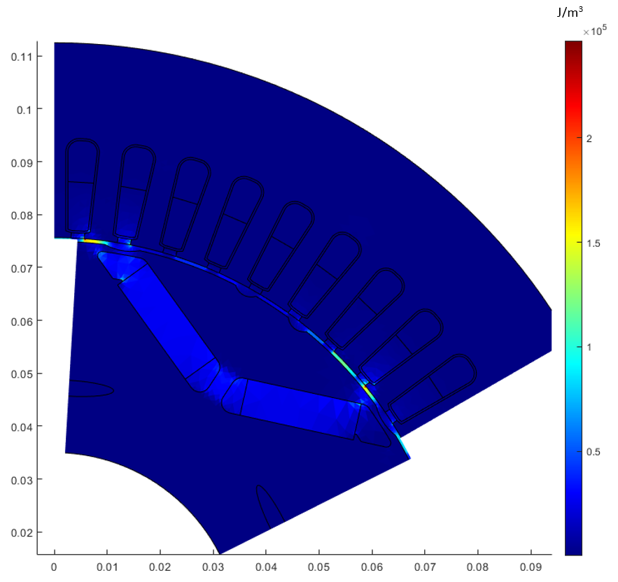
Let’s take a closer look at the magnetic field energy distribution in the cross section of the Tesla Model 3 motor, as depicted in Figure 1. As can be seen, the majority of the energy is concentrated in the air gap. From this observation, a straightforward conclusion can be drawn: in order to increase the power density of the motor while using weaker magnets, we need to expand the surface area of the air gap. To achieve this without increasing the overall motor size, we propose transitioning to an axial flux motor topology and employing multiple motors on the same shaft, with their combined weight matching that of the Tesla Model 3 motor.
Following this design approach, we utilized MotorXP-AFM, a specialized software dedicated to axial flux machine design and analysis. This allowed us to assess various axial flux motor structures and configurations to find the most suitable one for our objective. This process resulted in more than ten thousand individual designs evaluated, which can be categorized as presented in Table 2. Thanks to the implementation of super-fast quasi-3D FEA and advanced optimization algorithm, which enables efficient exploration of large design spaces, this entire process was completed in approximately 8 weeks. Each day, the software evaluated between 200 to 500 individual designs.
Table 2. Motor configurations explored in the first stage of the design process.
Design properties |
Explored configurations |
Selected configuration |
| Axial flux motor topology | stator-rotor-stator, rotor-stator-rotor | rotor-stator-rotor |
| Pole number | 10 poles, 14 poles, 20 poles | 14 poles |
| Number of motors on the shaft | 1, 2, 3, 4, 5 | 3 |
| Rotor magnet arrangement | Conventional South-North, Halbach arrays with different magnetization steps | Halbach array with 10 degrees magnetization step |
Task definition
Now, let’s define the task of this study. Our goal is to design a feasible permanent magnet motor using ferrite magnets, with the aim of closely matching the Tesla Model 3 motor in terms of weight, size, power, and efficiency under the same operating conditions. To achieve this, we started with the initial design data that remains consistent for both the Tesla Model 3 motor and the designed motor, as shown in Table 3.
|
Table 3. Initial design data. |
|
Parameter |
Value |
| Outer diameter of the core | 225 mm |
| Air gap | 0.7 mm |
| Core material | M-19 29 Ga |
| Winding material | Copper |
| Winding temperature | 80°C |
| Magnet temperature | 60°C |
| Slot fill factor | 0.3 |
| Core stacking factor | 0.95 |
The design process consists of two distinct stages. In the first stage, the motor configuration and the approximate dimensions are established to meet specified weight and efficiency requirements, while also preventing magnet demagnetization. In the second stage, the motor’s dimensions are further refined to establish the desired field-weakening capabilities, ensuring high efficiency across the entire operational range, all while adhering to weight, efficiency, and demagnetization criteria.
First stage of the design process: large-scale design space exploration
The design process involves exploring each motor configuration listed in Table 2. To do this, we set up an optimization algorithm for every motor configuration defining optimization objectives and a set of design variables, which represent the geometry dimensions in this case, along with their respective ranges (minimum and maximum values). In this stage, the optimization objectives remain consistent for all motor configurations and are presented in Table 4. However, the design variables and their ranges may differ depending on the specific motor configuration under investigation.
The optimization is carried out for each motor configuration of Table 2. In this stage, which we call large-scale design space exploration, we allow the design variables to vary over a relatively wide range. The primary aim is to assess whether the desired optimization objectives can be achieved for each particular motor configuration while adhering to the given constraints. This process is repeated for all the suggested motor configurations listed in Table 2.
After conducting this exploration for each motor configuration, we identified the most suitable configuration, which turned out to be the rotor-stator-rotor topology with a yokeless stator with 14 poles and a 10-degree step Halbach array rotors, consisting of three motors on the shaft. This chosen configuration is referred to as the “Selected configuration” and is listed in Table 2. Table 5 presents the design variables and their respective limits, specifically tailored for the optimization process of the selected motor configuration. Other motor configurations (see Table 2) explored in the first stage of the design process may have different design variables and are not presented in this article. The optimization is performed with a focus on three primary objectives: minimizing motor weight, minimizing losses during maximum power operation, and minimizing the permanent magnet demagnetization risk, as outlined in Table 4.
Table 4. Optimization objectives for the first stage of the design process.
Objective |
Target |
| Minimizing motor weight | 32,092 grams or less (divided by the number of motors on the shaft) |
| Minimizing losses (@ 430 Nm, 4275 RPM) | 16,330 Watts or less (divided by the number of motors on the shaft) |
| Minimizing the demagnetizing field (@ 430 Nm, 4275 RPM) | 310 kA/m or less |
Table 5. Ranges for the optimized geometry parameters for the selected motor configuration.
Design variable |
Minimum value |
Maximum value |
| Core inner diameter, [mm] | 110 | 170 |
| Slot width, [mm] | 10 | 30 |
| Slot height, [mm] | 20 | 67 |
| Slot opening width, [ratio to slot width] | 0.1 | 1 |
| Slot opening height, [mm] | 1 | 5 |
| Magnet height, [mm] | 5 | 25 |
| Rotor yoke height, [mm] | 1 | 5 |
The outcome of the design space exploration, carried out using the MotorXP-AFM optimization algorithm for the selected motor configuration, is displayed in Figure 2 as a Pareto plot. Each point on the graph represents a specific design location in the coordinate system of the three optimization objectives. The reference design × corresponds to the weight and losses of the Tesla Model 3 motor, divided by three, as there are three designed motors on the shaft. Based on these results, the most promising design candidate was selected for further analysis and optimization, as shown in Figure 2.
click on image to enlarge

Second stage of the design process: optimizing field-weakening operation
In challenging tasks like this, the large-scale design space exploration often doesn’t yield the most optimized design directly. However, it helps to narrow down the search space for the next round of the optimization process. Although the design selected in the previous section meets the targeted optimization objectives, it was found to underperform in the field-weakening region, which significantly reduced the overall motor efficiency.
To improve the field-weakening operation of the designed motor, we set up an optimization algorithm for the previously selected motor configuration introducing an additional objective of minimizing the characteristic current of the motor. Based on geometry dimensions of the design which we selected in the previous section, we also reduced the number of design variables and narrowed down their limits. The corresponding optimization objectives are listed in Table 6, while the geometry parameters are presented in Tables 7 and 8. This approach aims to further optimize the motor’s performance, with a specific focus on improving its field-weakening capabilities.
Table 6. Optimization objectives for the second stage of the design process (3 motors on the shaft are assumed).
Objective |
Target |
| Minimizing losses (@ 143.33 Nm, 4275 RPM) | 5443 Watts or less |
| Minimizing the demagnetizing field (@ 143.33 Nm, 4275 RPM) | 310 kA/m or less |
| Minimizing characteristic current to rated current ratio | 0.93 or less |
Table 7. Constant geometry parameters for the second stage of the design process.
Geometry parameter |
Value |
| Core outer diameter, [mm] | 225 |
| Core inner diameter, [mm] | 126.3 |
| Rotor yoke height, [mm] | 1.5 |
| Motor weight, [grams] | 10697 |
Table 8. Ranges for the optimized geometry parameters for the second stage of the design process.
Design variable |
Minimum value |
Maximum value |
| Slot width, [mm] | 13 | 21 |
| Slot height, [mm] | 22 | 37 |
| Slot opening width, [ratio to slot width] | 0.1 | 1 |
| Slot opening height, [mm] | 1 | 5 |
| Magnet height, [mm] | Determined to maintain motor weight of 10697 grams | |
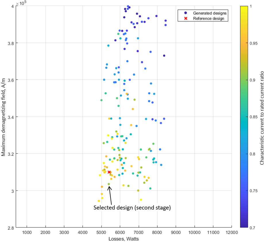
The characteristic current determines the motor’s ability to maintain a constant output power during the field-weakening operation. To simplify the optimization setup, we use a ratio of the characteristic current to the current at which the maximum torque is achieved. For the Tesla Model 3 motor, this ratio was determined to be 0.93. Therefore, to achieve the field-weakening capabilities for the designed motor similar to that of the Tesla Model 3 motor, we target a value of 0.93 or slightly lower for this optimization objective (see Table 6).
Notably, we excluded motor weight from the optimization objectives. Instead, the motor weight is now listed in Table 7 as a constant parameter. We achieve this by recalculating the magnet height once the other variable geometry parameters from Table 8 are set. This adjustment allowed us to reduce the number of optimization objectives while still maintaining the desired motor weight.
Figure 3 displays the Pareto plot of the second stage optimization results along with the final selected design. In Figure 4, you can see the final axial flux motor design, including its geometry, materials and winding parameters. As previously mentioned, there are three of these motors installed on the same shaft.
click on image to enlarge
click on image to enlarge
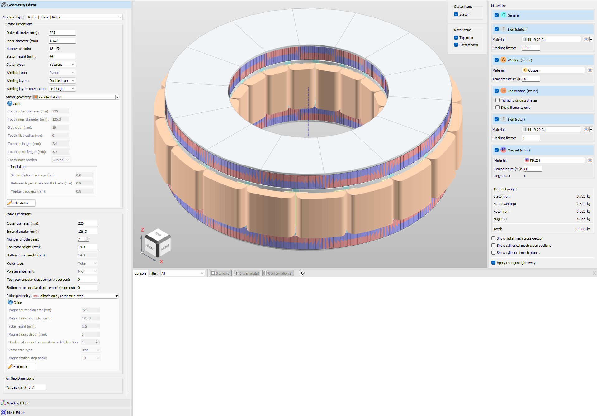
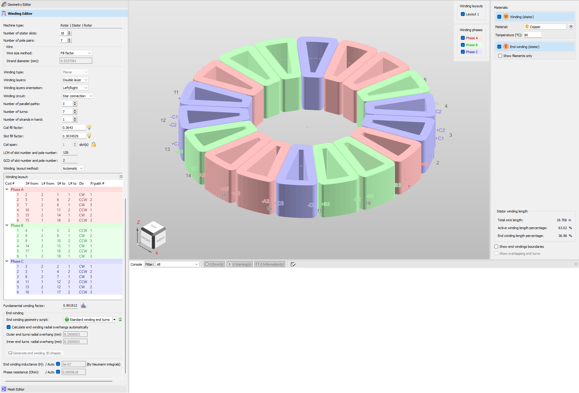
Figure 4. Final axial flux motor design: MotorXP-AFM Geometry Editor view (left) and Winding Editor view (right).
Comparison of the Tesla Model 3 motor and the designed motor characteristics
Table 9 presents a comparison of the size and weight characteristics between the Tesla Model 3 motor and the designed motor. While the weight of both motors is nearly identical, the designed motor is only slightly longer than the Tesla Model 3 motor. It’s worth noting that the designed motor requires significantly more magnets, over five times as many as the Tesla Model 3 motor, to compensate for the weakness of the ferrite magnets.
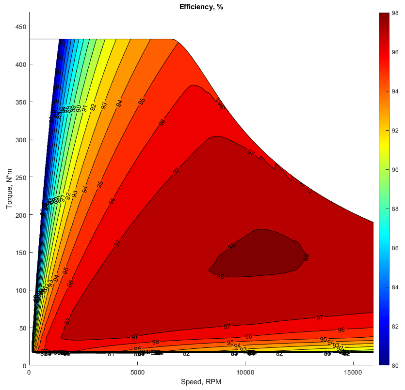
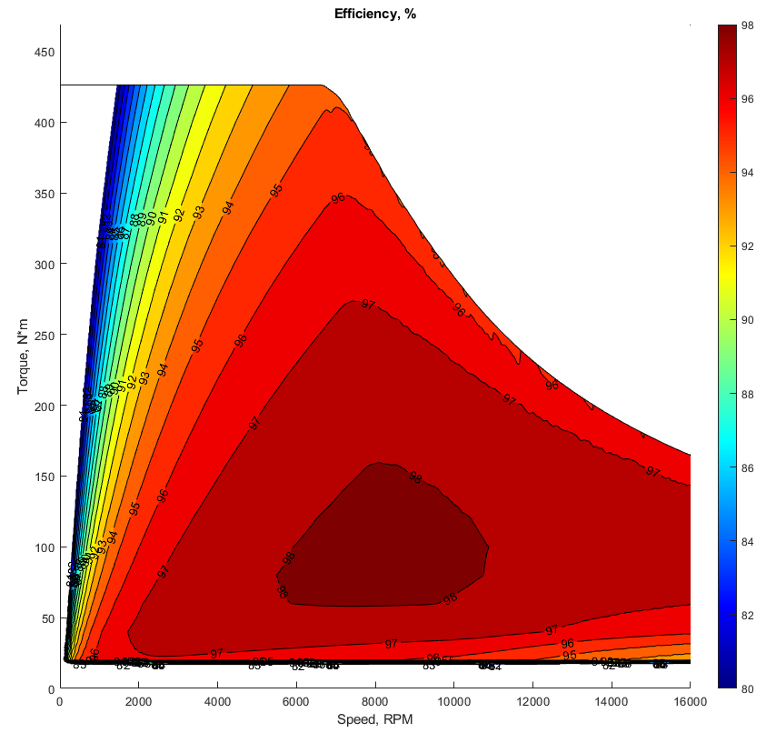
Tables 10 and 11 provide a comparison of the performance characteristics of the two motors at peak power and peak efficiency operation. Additionally, Figures 5 and 6 display the efficiency maps of the two motors for the same speed and load ranges. Notably, both motors exhibit nearly the same calculated peak efficiency, which is around 98%. However, for the Tesla Model 3 motor, the peak efficiency occurs at a lower speed and torque, as indicated in Table 11 and the presented efficiency maps (Figures 10 and 11). This can be attributed to the Tesla Model 3 motor’s superior field weakening capabilities, resulting from a significant reluctance torque component, which is typically low for motors with surface-mounted magnets, as is the case with the designed motor.
Table 9. Size and weight comparison.
Parameter |
Tesla Model 3 motor |
Designed motor (3 motors on the shaft) |
| Motor weight (active materials), kg | 32.092 | 32.040 |
| Motor length (active materials), mm | 214 (with end turns) | 222 |
| Outer diameter of the core, mm | 225 | 225 |
| Air gap, mm | 0.7 | 0.7 |
| Core weight, kg | 26.712 | 13.05 |
| Copper weight, kg | 3.506 | 8.532 |
| Magnet weight, kg | 1.874 | 10.458 |
Table 10. Comparison at peak power and peak torque operation.
Parameter |
Tesla Model 3 motor |
Designed motor (3 motors on the shaft) |
| Torque, Nm | 431.69 | 430.15 |
| Speed, RPM | 4275 | 4275 |
| Mechanical power, kW | 193.26 | 192.57 |
| Phase current, Arms | 942 | 1324 |
| Advance angle, el.deg. | 55 | 0 |
| Phase voltage, Vrms | 93.83 | 91.72 |
| Current density, A/mm2 | 43.29 | 27.29 |
| Power factor | 0.79 | 0.57 |
| Total losses (copper+iron+magnet), kW | 16.33 | 16.20 |
| Efficiency (without mechanical losses), % | 92.21 | 92.24 |
| Torque ripple (without skewing), % | 7.77 | 1.26 |
Table 11. Comparison at peak efficiency operation.
Parameter |
Tesla Model 3 motor |
Designed motor (3 motors on the shaft) |
| Torque, Nm | 102.40 | 146.90 |
| Speed, RPM | 8520 | 11355 |
| Mechanical power, kW | 91.36 | 174.68 |
| Phase current, Arms | 220 | 432 |
| Advance angle, el.deg. | 41 | 21 |
| Phase voltage, Vrms | 141.0 | 138.14 |
| Current density, A/mm2 | 10.11 | 8.90 |
| Power factor | 0.99 | 0.98 |
| Total losses (copper+iron+magnet), kW | 2.07 | 3.71 |
| Efficiency (without mechanical losses), % | 97.79 | 97.92 |
| Torque ripple (without skewing), % | 30.66 | 1.57 |
click on image to enlarge
click on image to enlarge
Validation with full 3D FEA
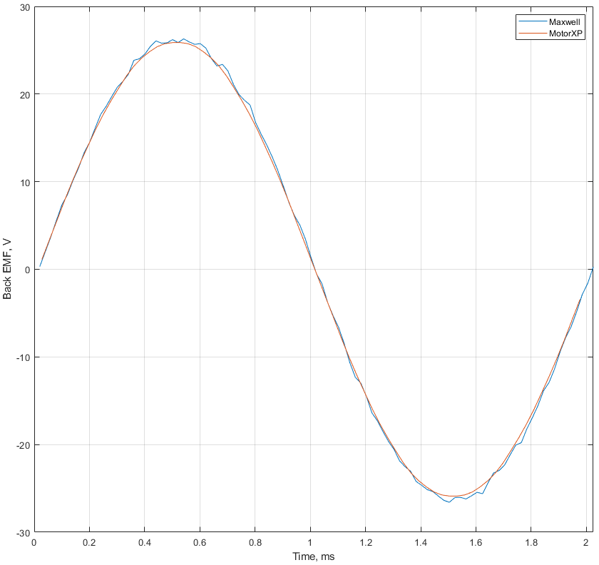
While MotorXP-AFM provides fast and reliable results based on quasi-3D FEA, we strongly recommend using full 3D FEA software for the final validation. In this study, we used ANSYS Maxwell 3D to validate the primary calculations performed with MotorXP-AFM. Figure 7 displays the no-load back EMF waveform calculated in MotorXP-AFM at a speed of 4275 RPM, compared with the back EMF waveform calculated in ANSYS Maxwell at the same speed. Figure 8 presents a comparison of the torque waveforms calculated at a speed of 4275 RPM and RMS stator current of 1324 A. For a summarized overview of the back EMF and torque comparison, please refer to Table 12.
click on image to enlarge
click on image to enlarge
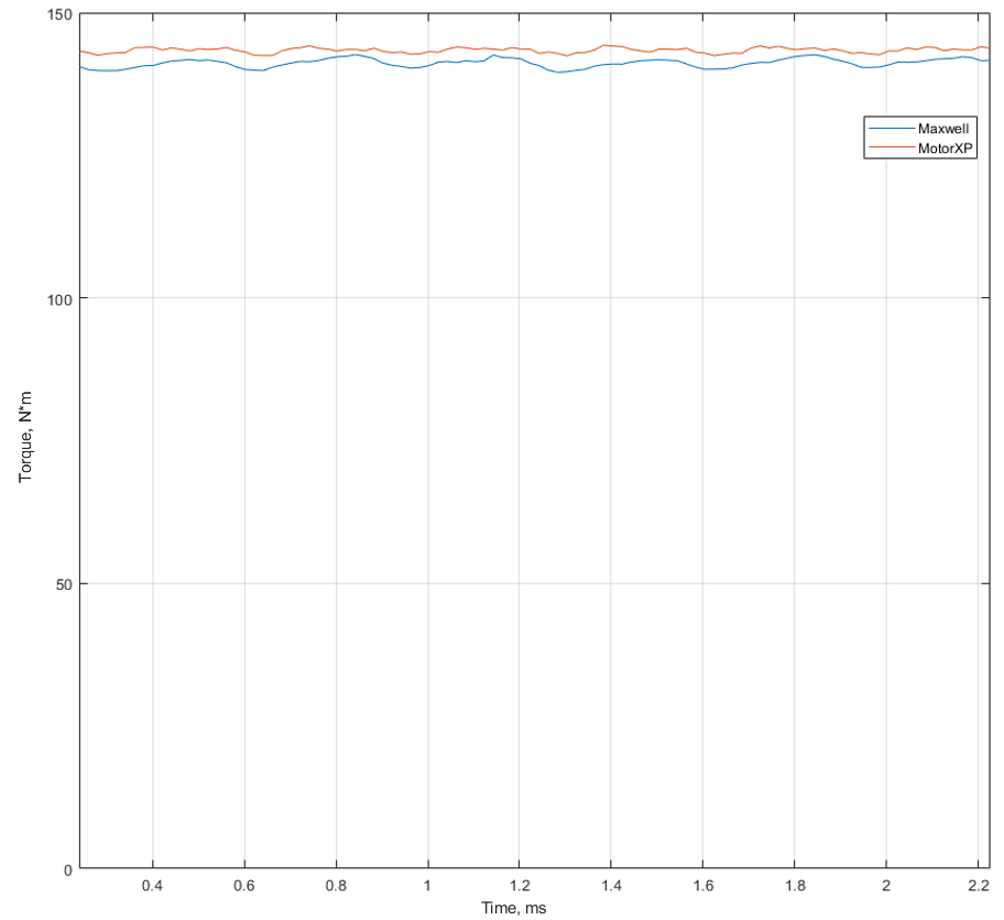
Figure 8. Comparison of torque waveforms calculated in MotorXP-AFM and ANSYS Maxwell.
Table 12. MotorXP-AFM vs. ANSYS Maxwell 3D back EMF and torque comparison.
Parameter |
ANSYS Maxwell 3D |
MotorXP-AFM |
Discrepancy, % |
| Back EMF peak, V (@ 4275 RPM) | 26.3 | 25.9 | 1.52 |
| Torque, N*m (@ 4275 RPM, 1324 Arms) | 141.2 | 143.4 | 1.56 |
Before delving into the comparison of iron losses, it’s important to understand how iron losses are calculated in both MotorXP-AFM and ANSYS Maxwell. Despite both programs utilizing the same Steinmetz equation:
\(P = K_h f^\alpha B_m^\beta + K_e (f \cdot B_m)^2\) ,
there are differences in the iron loss coefficients they employ, which are outlined in Table 13.
In the Steinmetz equation, the first term accounts for hysteresis losses, while the second term represents eddy current losses. The coefficients Kh, α, β, and Ke are determined through fitting the equation to manufacturer-supplied iron loss data at various frequencies.
Table 13. Steinmetz equation iron loss coefficients for M-19 29 Ga steel used by MotorXP-AFM and ANSYS Maxwell.
Coefficient |
MotorXP-AFM |
ANSYS Maxwell 3D |
| Kh | 0.0113808 | 0.0287582 |
| α | 1.14987 | 1 |
| β | 1.76216 | 2 |
| Ke | 4.67093e-05 | 5.22876e-05 |
To facilitate a fair comparison, Table 14 presents the iron losses calculated in MotorXP-AFM using two sets of coefficients listed in Table 13. Notably, when using Maxwell’s coefficients, the difference in iron losses between calculations in ANSYS Maxwell and MotorXP-AFM remains within a 10% range. This discrepancy can be attributed to additional iron losses stemming from stator winding end turns, which are not factored into the MotorXP-AFM 2D iron loss model. In practical terms, this level of difference is generally acceptable for making informed design decisions.
Table 14. MotorXP-AFM vs. ANSYS Maxwell 3D iron losses comparison.
 |
ANSYS Maxwell 3D |
MotorXP-AFM (MotorXP coefficients) |
Discrepancy with MotorXP coefficients, % |
MotorXP-AFM (Maxwell coefficients) |
Discrepancy with Maxwell coefficients, % |
| Iron losses at no-load, W | 138.7 | 152.1 | 9.6% | 163.1 | 17.6% |
| Iron losses under load, W | 413.7 | 341.1 | 17.6% | 373.9 | 9.6% |
Challenges and Considerations in Manufacturability, Mechanical, and Thermal Aspects
As previously mentioned, this study primarily focuses on electromagnetic design, with other aspects receiving only brief discussion without deep analysis.
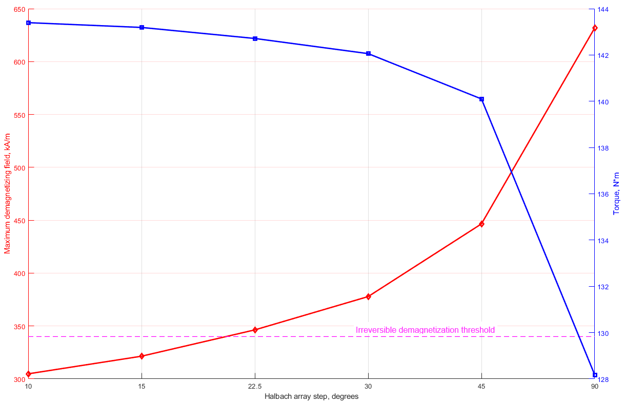
Balancing demagnetization resistance of the permanent magnets with high power density of the motor and suitable field-weakening capabilities posed the most significant challenge in this study. The resulting design incorporates a rotor with a 10-degree magnetization step Halbach array. Figure 4 illustrates each rotor consisting of 252 magnet pieces, each magnetized in various directions and then assembled to achieve the desired Halbach array with the appropriate magnetization step. This assembly process may raise significant manufacturing challenges. However, the use of the Halbach array with such a high number of components is necessitated by requirements for permanent magnet demagnetization resistance. Reducing the Halbach array magnetization step significantly decreases the demagnetizing field, as demonstrated in Figure 9. According to Figure 9 to surpass the irreversible demagnetization threshold, a minimum 15-degree magnetization step is required for the Halbach array in this case, but a 10-degree step was chosen to provide a 10% margin for the demagnetizing field.
click on image to enlarge
Increasing the Halbach array magnetization step and addressing associated manufacturing challenges could be achieved by increasing the motor’s diameter so that the required torque could be generated with lower current and a reduced demagnetizing field. This could be a good practical solution, but, since the motor’s diameter is constrained by the task statement, this option was not considered in this study. Another potential solution might involve a single-piece Halbach array with “continuously changing magnetization”.
The increased rotor diameter of the designed axial flux motor, compared to the Tesla Model 3 motor, could potentially limit the motor’s maximum speed. Additionally, the surface-mounted structure of the designed motor is less mechanically robust compared to the interior permanent magnet structure used in the Tesla Model 3 motor. This might necessitate additional measures, such as a carbon fiber retaining sleeve, to reinforce the rotor.
Using three motors on the same shaft, unlike the single motor configuration of the Tesla Model 3 motor, along with the yokeless stator structure in the designed motor, may complicate the cooling process. However, the increased copper weight in the designed motor will enhance thermal inertia and improve heat dissipation due to a larger winding surface area.
Conclusion
This study demonstrates the feasibility of designing a permanent-magnet motor using ferrite magnets that rivals the efficiency and power density of the Tesla Model 3 motor from an electromagnetic perspective. While the designed motor may present challenges related to manufacturability, mechanical aspects, and cooling, it’s important to note that these issues fall outside the scope of this study.
The utilization of modern optimization algorithms, coupled with parallel processing and state-of-the-art simulation technologies, represents a powerful tool for motor design engineers. It eliminates the need for days of monotonous work of manual parameter adjustments, providing more room for creativity and substantially reducing man-hours through automation of the design process. This advancement elevates motor design to an entirely new level, enabling the achievement of design objectives that were once deemed unattainable.
Related articles
From Simulation-Driven to Optimization-Driven Electric Motor Design
Overview of the automatic electric motor optimization using the MotorXP software. Read article>>
AI-powered electric motor design
Practical implementation of the automatic motor design workflow using the automatic optimization features of the MotorXP software. Read article>>