3D FEA is the most used technique for simulation of axial flux machines (AFM) due to their intrinsic 3D magnetic structure. But these simulations are extremely time consuming especially at initial design stages. There is also a well-know 2D FEA technique when the AFM is represented by one or several linear machines with equivalent topologies by slicing the 3D geometry of the AFM with cylindrical planes of different radii (2D Linear Machine Modeling Approach – 2D-LMMA [1]) as shown in Figure 1. Then the magnetic field problem is solved in each slice all at the same time with 2D FEM. The electromagnetic torque is calculated for every slice and the actual torque is obtained as a summation of all slice values.
The main drawback of 2D-LMMA is limited accuracy due to strong influence of 3D effects on the AFM performance. To include 3D effects into 2D-LMMA, MotorXP-AFM also computes the magnetic field in the radial cross-section of the AFM and uses geometry correction coefficients to take into account the exact shape of different parts of the machine. Example of the radial cross-section mesh of the AFM is shown in Figure 2.
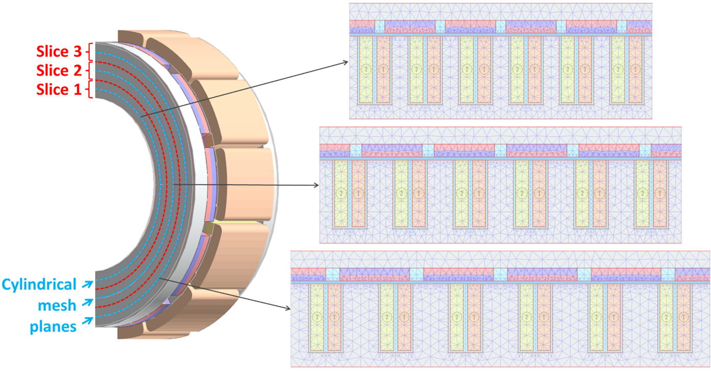
Figure 1. Axial flux machine 2D Linear Machine Modeling Approach (2D-LMMA) with three cylindrical mesh slices.
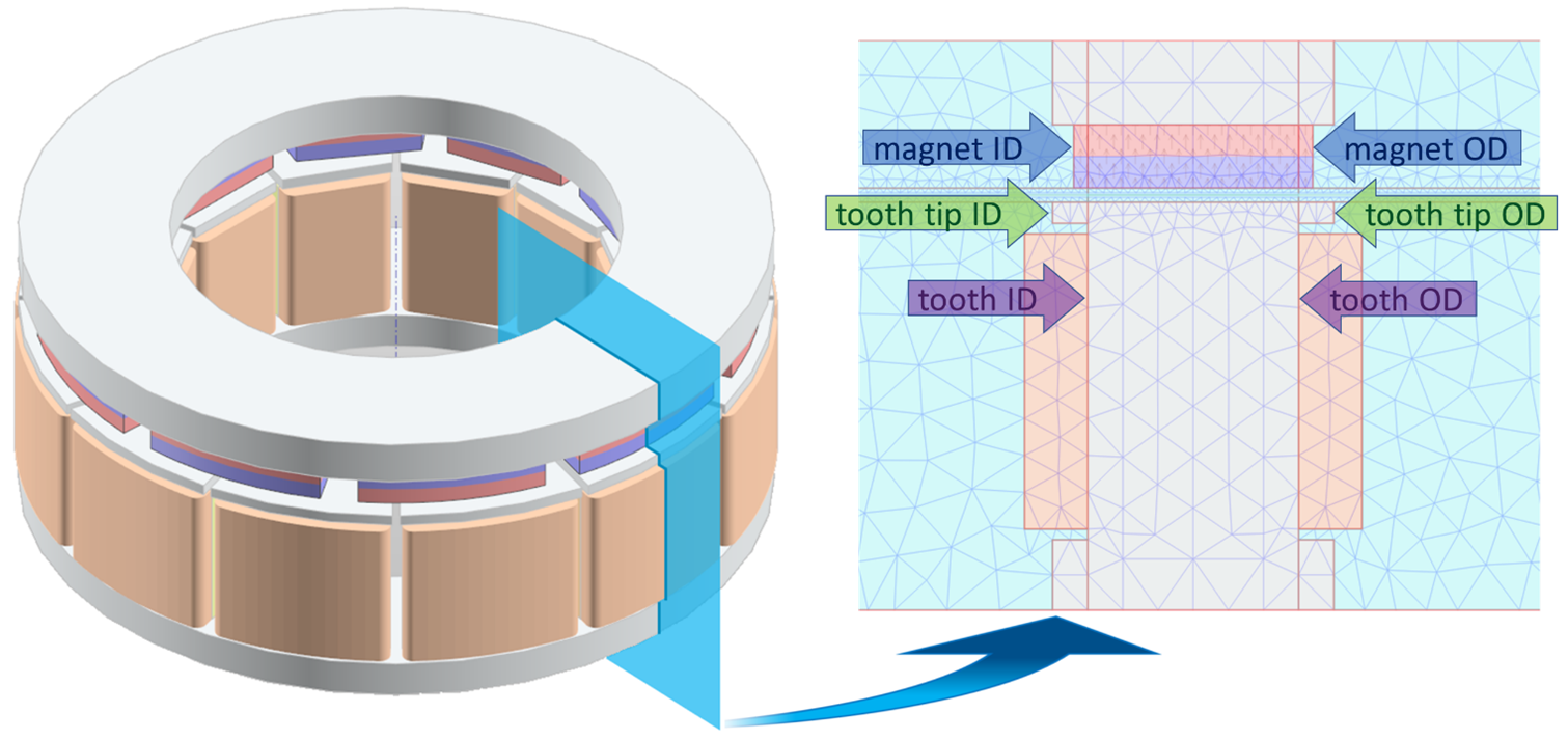
Figure 2. Axial flux machine radial cross-section mesh.
The magnetic field of the AFM can be divided into circumferential and radial components. The circumferential component of the magnetic field is the one observed in the cylindrical cross-sections as shown in Figure 1 and can be accurately calculated by using 2D-LMMA. The radial component of the magnetic field is the one observed in the radial cross-sections as shown in Figure 2. The radial component is mostly determined by the end effects, such as the leakage flux alone the radial cross-section plane and a variation of the inner and outer diameters of different parts of the AFM. The radial component of the magnetic field and the associated 3D effects are not directly included into 2D-LMMA but can be taken into account by also considering the magnetic field in the radial cross-section of the AFM. For example, Figure 2 shows AFM having different inner and outer diameters of stator teeth, rotor magnets and tooth tips. Magnetic field solution in the radial cross-section allows to consider the effect of these geometry characteristics on the AFM performance.
In order to reduce the number of machine cross-sections without scarifying the accuracy while taking into account most of the 3D geometry details, the geometry correction coefficients are used. Figures 3 and 4 show some examples of geometry details which are taken into account through the geometry correction coefficients. The geometry correction coefficients are automatically calculated for different parts of the AFM (rotor and stator back iron, tooth, magnet, and tooth tip) and incorporated into the AFM model.
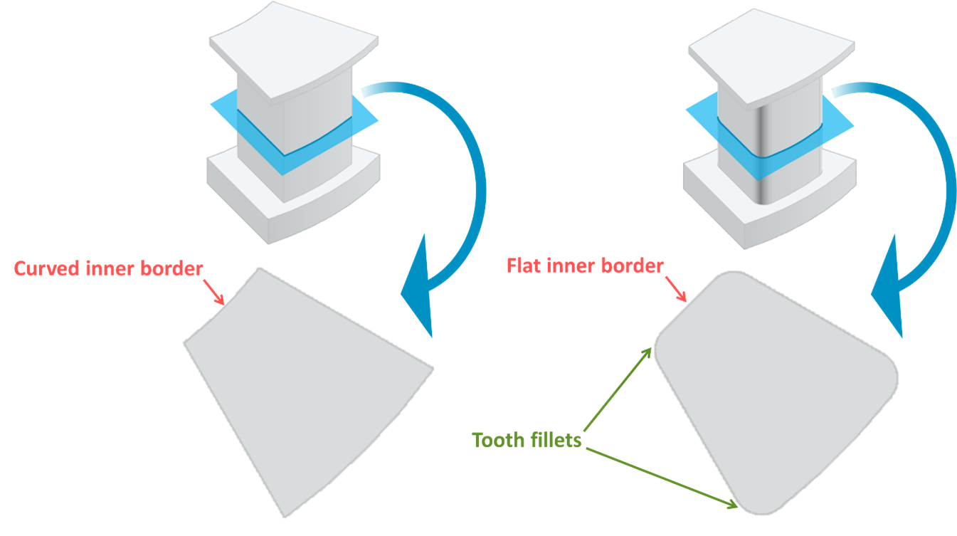
Figure 3. Examples of two stator tooth shapes which are taken into account using geometry correction coefficients.
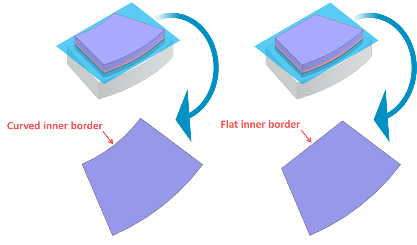
Figure 4. Examples of two rotor magnet shapes which are taken into account using geometry correction coefficients.
References
[1] Gulec, M.; Aydin, M. Implementation of different 2-D finite element modelling approaches in axial flux permanent magnet disc machines. IET Electr. Power Appl. 2018, 12, 195–202.